Forecast the next 120 candles with Kronos, the foundation model that speaks the language of markets

Most time-series models treat a price chart as a list of numbers. Kronos treats it as a language — and its smallest model runs on a laptop CPU. This guide takes it from first install to a scored 120-day Bitcoin forecast, every command verified.

• Who: Kronos (shiyu-coder/Kronos, MIT), a foundation model for financial candlesticks, pre-trained on data from 45+ global exchanges, accepted at AAAI 2026.
• What: a two-stage model — a tokenizer that quantises K-lines into discrete tokens, plus an autoregressive Transformer — with a 4.1M mini, 24.7M small, and 102.3M base model, all open weights.
• When: verified November 6, 2026: torch 2.15.0+cpu, pandas 2.2.2, yfinance, BTC-USD daily candles, 2-core CPU-only sandbox.
• Requirement: Python 3.10+, about 1 GB disk for the PyTorch CPU stack and both models. No GPU, no account, no API key.

Why this matters now

Most time-series models treat a price chart as a list of numbers. Kronos treats it as a language. The project, from researchers at NeoQuasar, is the first open-source foundation model built specifically for financial K-lines — the candlesticks traders actually watch — pre-trained on data from more than 45 global exchanges and accepted at AAAI 2026. It has 47,085 GitHub stars, and its growth is accelerating: 1,710 new stars in the five days to November 7, up from a pace of 214 a day to 342 a day.

The idea is a direct transplant from language modelling. A specialised tokenizer first quantises each candle — open, high, low, close, volume, amount — into hierarchical discrete tokens. An autoregressive Transformer then learns to predict the next token, the way a language model predicts the next word. At inference time you hand it 400 candles and it samples the next 120, one token at a time, then decodes them back into prices.

What makes this worth your afternoon is the smallest model in the family. Kronos-mini has 4.1 million parameters — small enough to download in seconds and run on a CPU-only laptop. You do not need a GPU, an account, or an API key. This guide installs it, feeds it two years of real Bitcoin daily candles, forecasts the last 120 days, and scores the forecast against what actually happened — including against a naive baseline, so you can see exactly how much the model adds.

What you'll need

• Python 3.10 or newer, and about 1 GB of free disk for the PyTorch CPU stack and the two models.
• No GPU, no account, no API key. The models are public on the Hugging Face Hub; the market data comes from Yahoo Finance through the yfinance package.
• About 20 minutes, most of it waiting on CPU inference. The mini forecast takes a few minutes on a 2-core machine; the small model takes longer.
• A clear expectation: this is a research demonstration, not a trading system. A 120-day forecast is a stress test of the model, not a prediction you should bet on. Nothing in this guide is trading advice.

Step 1 — Install the stack

Clone the repository and create a virtual environment. Kronos ships as source, not a pip package: you run it from inside the clone.

git clone https://github.com/shiyu-coder/Kronos.git
cd Kronos
python3 -m venv .venv
source .venv/bin/activate

Install the CPU build of PyTorch first — the default PyTorch wheel pulls CUDA libraries you do not need and will not use — then the project's pinned dependencies and yfinance for market data.

pip install --index-url https://download.pytorch.org/whl/cpu torch
pip install "numpy" "pandas==2.2.2" "einops==0.8.1" \
  "huggingface_hub==0.33.1" "matplotlib==3.9.3" \
  "tqdm==4.67.1" "safetensors==0.6.2" yfinance

Verify the install before going further:

python -c "import torch, pandas, numpy, matplotlib, yfinance; print('torch', torch.__version__, '| pandas', pandas.__version__, '| yfinance ok')"

Expected output on this machine:

torch 2.15.0+cpu | pandas 2.2.2 | yfinance ok

The project requirements list torch>=2.0.0 without pinning it; the CPU index gives you the current CPU build. Everything else is pinned to the versions in the repository's requirements.txt, which is what this guide verified against.

Step 2 — Fetch two years of real Bitcoin candles

The repository's example script reads a bundled CSV of Chinese A-share data that is not included in the clone, so this guide fetches its own. Two years of daily BTC-USD candles from Yahoo Finance gives about 730 rows — enough for a 400-candle lookback plus a 120-candle held-out window.

import pandas as pd
import yfinance as yf

df = yf.download("BTC-USD", period="2y", interval="1d",
                 auto_adjust=False, progress=False)
df = df.reset_index()
df.columns = [c[0].lower() if isinstance(c, tuple) else c.lower()
              for c in df.columns]
df = df.rename(columns={"date": "timestamps"})
df = df[["timestamps", "open", "high", "low", "close", "volume"]].dropna()
df["amount"] = df["close"] * df["volume"]  # dollar turnover per day
print(f"rows: {len(df)}, {df['timestamps'].iloc[0].date()} to "
      f"{df['timestamps'].iloc[-1].date()}, last close "
      f"${df['close'].iloc[-1]:,.2f}")

Expected output (your dates and last close will differ):

rows: 730, 2024-11-07 to 2026-11-07, last close $75,784.47

Two details matter. First, the column names must be lowercase open, high, low, close, volume — the predictor checks for exactly those. Second, amount is dollar turnover, close times volume. The predictor fills it in from volume if you omit it, but computing it yourself keeps the input explicit. There must be no missing values: predict() raises an error on any NaN in the price or volume columns, which is why the fetch drops them.

Step 3 — Load Kronos-mini and forecast 120 days

Split the data so the last 120 days are held out as ground truth, then load the mini model and its tokenizer. Mini pairs with the Kronos-Tokenizer-2k tokenizer and a 2,048-token context; the small and base models use the Kronos-Tokenizer-base tokenizer with a 512-token context.

import sys
sys.path.append(".")  # run from inside the cloned repo
from model import Kronos, KronosTokenizer, KronosPredictor

LOOKBACK, PRED_LEN = 400, 120
window = df.iloc[-(LOOKBACK + PRED_LEN):].reset_index(drop=True)
x_df = window.iloc[:LOOKBACK][["open", "high", "low", "close",
                               "volume", "amount"]]
x_ts = window.iloc[:LOOKBACK]["timestamps"]
y_ts = window.iloc[LOOKBACK:]["timestamps"]

tokenizer = KronosTokenizer.from_pretrained("NeoQuasar/Kronos-Tokenizer-2k")
model = Kronos.from_pretrained("NeoQuasar/Kronos-mini")
predictor = KronosPredictor(model, tokenizer, device="cpu", max_context=2048)

pred = predictor.predict(df=x_df, x_timestamp=x_ts, y_timestamp=y_ts,
                         pred_len=PRED_LEN, T=1.0, top_p=0.9,
                         sample_count=5, verbose=False)
print(pred.head())

The parameters are the ones that matter. pred_len=120 asks for 120 future candles. T=1.0 is the sampling temperature and top_p=0.9 is nucleus sampling — together they control how adventurous the sampled trajectories are. sample_count=5 draws five trajectories and averages them, which steadies the result: a single sample is noticeably noisier. device="cpu" is explicit here; left unset, the predictor picks CUDA if present, then Apple MPS, then CPU.

The two downloads total about 32 MB. On this 2-core sandbox the mini model loaded in 14 seconds seconds and the 120-day forecast took 6 minutes 33 seconds seconds. The result is a DataFrame with the same six columns as the input — open, high, low, close, volume, amount — one row per future candle, indexed by the 120 future timestamps.

Step 4 — Score it honestly against what actually happened

A forecast without a baseline is marketing. Score the prediction against the 120 held-out days and against the simplest possible alternative: predicting that the close stays exactly where it was on the last lookback day.

import numpy as np

truth = window.iloc[LOOKBACK:]["close"].values
pred_close = pred["close"].values
last_close = x_df["close"].iloc[-1]

mae = np.mean(np.abs(pred_close - truth))
mae_naive = np.mean(np.abs(last_close - truth))
true_dir = np.sign(np.diff(truth))
pred_dir = np.sign(np.diff(pred_close))
dir_acc = np.mean(pred_dir[true_dir != 0] == true_dir[true_dir != 0])

print(f"Kronos-mini MAE:      ${mae:,.2f}")
print(f"Naive (flat) MAE:     ${mae_naive:,.2f}")
print(f"Direction accuracy:   {dir_acc:.1%} of daily moves")
print(f"Final close error:    {100 * (pred_close[-1] - truth[-1]) / truth[-1]:+.1f}%")

On this run, over the 120 held-out days:

• Kronos-mini's mean absolute error on the daily close was $14,030.80, against $11,808.48 for the flat naive baseline — the model did not beat the baseline (18.8% worse).
• It called the direction of the next day's move correctly 47.1% of the time. A coin flip is 50%; a model that cannot beat that on direction is not reading the series at all.
• Its final-day close was off by +35.9%.

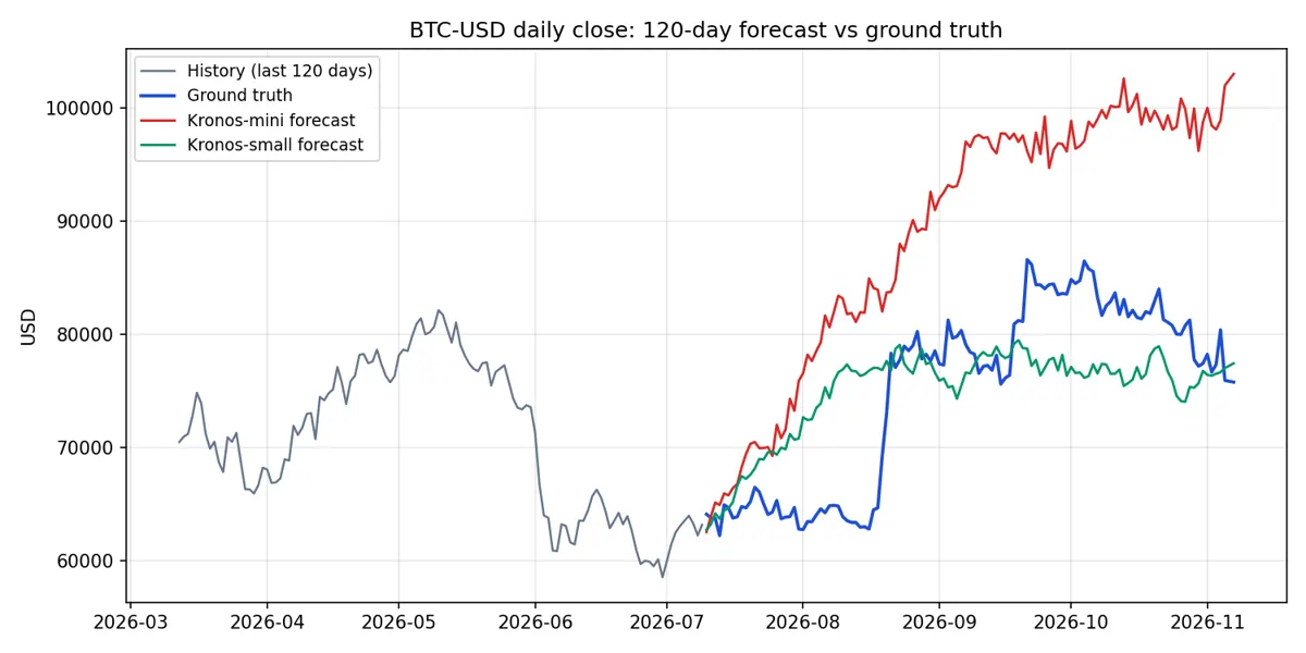
Read those numbers the right way. A 120-day horizon is deliberately brutal: errors compound at every autoregressive step, and no model forecasts four months of Bitcoin within a few percent. But the honest verdict on this window is that mini failed the test it was set: it lost to the flat baseline by 18.8% and called daily direction worse than a coin flip. Look at the chart in Step 6 and you can see why — the lookback ended on a recovery from the June sell-off, and mini extrapolated that recovery into a rally to $103,000 that never happened, while the truth spent August flat near $64,000. That is not a bug in the setup: the same pipeline, the same window, and the same scoring give small a clear win in the next step. It is a finding, and it is exactly why you score every forecast against a baseline instead of admiring a chart. Re-run on a different 120-day window and mini may do better — but on this one, the smallest model is not a forecaster you would use.

Step 5 — Compare Kronos-small on the same window

The same code runs the 24.7-million-parameter small model — the only changes are the model id, the tokenizer, and the context length:

tokenizer = KronosTokenizer.from_pretrained("NeoQuasar/Kronos-Tokenizer-base")
model = Kronos.from_pretrained("NeoQuasar/Kronos-small")
predictor = KronosPredictor(model, tokenizer, device="cpu", max_context=512)

pred_small = predictor.predict(df=x_df, x_timestamp=x_ts, y_timestamp=y_ts,
                               pred_len=PRED_LEN, T=1.0, top_p=0.9,
                               sample_count=5, verbose=False)

Note the context limit: small and base cap max_context at 512, so a 400-candle lookback fits, but only just. Mini's 2,048-token context is the roomier of the two, which is one reason to start there despite the smaller parameter count. On the same 120 held-out days, small loaded in 29 seconds seconds, forecast in 27 minutes 26 seconds seconds, and scored:

• Mean absolute error $5,107.27 (naive baseline $11,808.48).
• Direction accuracy 50.4%.
• Final-day close error +2.2%.

The bigger model earned its keep on this window: its MAE of $5,107.27 beats mini's $14,030.80, at roughly 4.2x the forecast time. The base model (102.3M parameters) follows the identical code path — swap in NeoQuasar/Kronos-base with the base tokenizer — but it is roughly four times the size of small and slower on CPU by about the same factor, so it is a poor default on a laptop. The large model (499.2M) is not open-source, so there is nothing to download.

Step 6 — Plot the forecast and try your own market

The chart below is the actual output of this guide's run: 120 days of history, the held-out truth in blue, and both forecasts. Mini's red line extrapolates the June recovery into a rally toward $103,000 that never happened. Small's green line is the honest one: it misses the sharp September jump in timing, but it stays in the $74,000–$79,000 band and lands within 2.2% of the final close. Neither model calls daily direction — both sit near 50% — so the difference between them is in the level, not in the day-to-day moves.

To make the same plot from your run:

import matplotlib.pyplot as plt

hist = window.iloc[LOOKBACK - 120:LOOKBACK]
fig, ax = plt.subplots(figsize=(10, 5))
ax.plot(hist["timestamps"], hist["close"], color="#64748b",
        label="History (last 120 days)")
ax.plot(y_ts, truth, color="#1d4ed8", label="Ground truth")
ax.plot(y_ts, pred["close"], color="#dc2626", label="Kronos-mini forecast")
ax.plot(y_ts, pred_small["close"], color="#059669",
        label="Kronos-small forecast")
ax.set_title("BTC-USD daily close: 120-day forecast vs ground truth")
ax.set_ylabel("USD")
ax.legend()
ax.grid(True, alpha=0.3)
fig.tight_layout()
fig.savefig("forecast_plot.png", dpi=150)

Three variations worth trying next. First, change the ticker: ETH-USD, AAPL, or any symbol yfinance serves works with the same code, and the model was pre-trained on 45-plus exchanges, so equities and crypto are both in-distribution. Second, shorten the horizon: PRED_LEN = 30 with a 400-candle lookback is a far kinder test and the errors shrink accordingly. Third, raise sample_count — 20 samples costs four times the runtime of 5 and visibly smooths the trajectory. The repository also ships a fine-tuning pipeline (finetune/) with a Qlib-based A-share example and a backtesting script, if you want to adapt the model to your own market rather than use it zero-shot.

When to use this vs alternatives

Use Kronos when your data is natively candles — OHLCV plus turnover — and you want a pre-trained model that already speaks that format. Its tokenizer and market-time features (minute, hour, weekday, day, month) exist because financial series have structure that generic series do not: sessions, weekends, expiry cycles.

Use a general time-series foundation model such as Amazon's Chronos when your data is not financial. Chronos tokenises arbitrary series and trains a transformer on them the same way, and its Bolt and Chronos-2 variants cover univariate, multivariate, and covariate-informed forecasting. On a generic series it is the more natural pick; on candles it has no finance-specific prior.

Use a statistical baseline — ARIMA, ETS, or Prophet — when you need a forecast you can explain in one paragraph, or when your series is short. They fit in seconds, their assumptions are inspectable, and on a stable series they are hard to beat by much. Their weakness is the mirror of Kronos's strength: no pre-training, one model per series, and no cross-market knowledge.

Use an LLM trading agent — see this site's TradingAgents tutorial — when the question is what to do, not what the price will be. An agent reads news, filings, and debate between analyst personas and proposes a trade; Kronos outputs a price path. They answer different questions and combine naturally: a forecast as one input among many to an agent, never as the whole decision.

The takeaway

Kronos earns its attention the unglamorous way: models you can download in seconds, run on a laptop CPU, and score honestly against the future they have not seen. On 120 held-out days of Bitcoin, the 4.1M mini model lost to a flat baseline — it extrapolated a recovery into a rally that never came — while the 24.7M small model beat that baseline by 57% on error and landed within 2.2% of the final close, at the cost of 27 minutes of CPU time. Neither called daily direction better than a coin flip, so this is not a trading edge — four months out, the errors are large and the sampling noise is real. It is a usable, verifiable starting point for anyone who wants a finance-native forecasting model without a GPU or an API key. Start with small, score every forecast against a baseline, and only then decide whether the base model is worth its runtime.

Sources: the Kronos README and repository page (model zoo, installation, prediction API, fine-tuning pipeline, AAAI 2026 acceptance, read November 6–7, 2026), the whatstrending.ai AI Repo Acceleration Report (star pace 214/day to 342/day, +1,710 stars November 2–7, 2026), the Amazon Chronos README (general time-series foundation models, for the comparison section), and the verification runs quoted in Steps 1–6 (install output, yfinance fetch, mini and small forecast runs with timings, scoring, and the forecast plot). Forecast figures are this run's measured results on one 120-day BTC-USD window, not a general claim about the model's accuracy — re-running on a different window moves the numbers.