Fine-tune embeddings for your domain: contrastive training that measurably improves retrieval
Generic embeddings rank the wrong document first on domain jargon. This tutorial fine-tunes all-MiniLM-L6-v2 with 60 contrastive pairs on a CPU in about 80 seconds — and measures accuracy@1 rising from 0.694 to 0.861 on held-out queries.

Your RAG pipeline's retriever is probably a generic embedding model trained on the open web. It knows what "bank" means in forty contexts, but it has never read your runbooks, your support macros, or your product's internal vocabulary. So when a user asks a question full of your domain's jargon, the retriever does something embarrassing: it ranks a document that sounds similar above the document that is the answer. The language model then confidently answers from the wrong context, and you get to debug a hallucination that was really a retrieval failure.
The fix is unfashionable and extremely effective: fine-tune the embedding model itself on your domain. Not a bigger model, not a fancier pipeline — the same small, fast bi-encoder, taught your vocabulary with a few dozen contrastive examples. In this tutorial you will do exactly that, end to end, on a CPU, with measurements at every step. The demo domain is 3D-printer troubleshooting Q&A (jargon-heavy, full of lookalike documents), the model is all-MiniLM-L6-v2, the training set is 60 question–answer pairs, and training takes about 80 seconds. The result: top-1 accuracy on held-out queries goes from 0.694 to 0.861, and MRR@10 from 0.814 to 0.926. Every number below was produced by running the code in this article — nothing is illustrative.
What you'll need#
- Python 3.10+ with
pip. Everything runs on CPU; a GPU makes it faster but changes nothing about the method. - Three packages:
sentence-transformers(6.x),datasets, andaccelerate(the trainer backend). About 200 MB of downloads for the base model. - No accounts, no API keys, no spending. The model and the data live on your machine.
- About 15 minutes, most of it waiting on
pipand the 80-second training run.
The workflow has six steps: build an evaluation set first, measure the baseline, assemble contrastive training pairs, train, measure the gain, and ship the model. The order matters — step one exists so that step five means something.
Step 1: Build your evaluation set first#
Never fine-tune without a way to know whether it worked. Before touching any training code, assemble a small corpus of documents in your domain and a set of test queries whose correct answers you know — written in different words from anything the model will train on. If your test queries overlap your training pairs, you will measure memorization, not retrieval.
For this tutorial the corpus is 12 troubleshooting documents (stringing, heat creep, first-layer adhesion, warping, under-extrusion, and seven more), each a few sentences long. The vocabulary deliberately overlaps across documents — "temperature", "nozzle", and "retraction" appear in half of them — because that is exactly where generic embeddings fail. The test set is 36 queries, three per document, each paraphrased differently from the training questions. One example: the training questions for heat creep ask about "extrusion dying 30 minutes into a print", while a test query asks "extruder clicking and no filament coming out after 20 minutes of printing?" — sharing the words "clicking" and "no filament" with the clogged nozzle document, a deliberate trap.
The metrics are the two that matter for retrieval:
- Accuracy@1: the fraction of queries where the correct document is ranked first. This is the number your users feel.
- MRR@10 (mean reciprocal rank): the average of 1 / (rank of the correct doc), counting only ranks up to 10. It rewards "close" even when the top hit is wrong.
Here is the evaluator. It encodes the corpus once, encodes each query, ranks by cosine similarity, and reports both metrics:
import numpy as np
from sentence_transformers import SentenceTransformer

def evaluate(model, docs, test_pairs):
    doc_ids = list(docs.keys())
    doc_emb = model.encode(
        [docs[i] for i in doc_ids],
        normalize_embeddings=True, show_progress_bar=False,
    )
    q_emb = model.encode(
        [q for q, _ in test_pairs],
        normalize_embeddings=True, show_progress_bar=False,
    )
    sims = q_emb @ doc_emb.T  # cosine similarity, since vectors are normalized
    acc1, mrr = 0, 0.0
    for row, (_, gold) in zip(sims, test_pairs):
        rank = int(np.where(np.argsort(-row) == doc_ids.index(gold))[0][0]) + 1
        if rank == 1:
            acc1 += 1
        if rank <= 10:
            mrr += 1.0 / rank
    n = len(test_pairs)
    return {"accuracy@1": acc1 / n, "mrr@10": mrr / n}

docs = {...}        # doc_id -> document text (12 docs)
test_pairs = [...]  # (query, correct_doc_id) (36 held-out queries)
Two details worth keeping. First, normalize_embeddings=True turns the dot product into cosine similarity — the standard comparison for these models. Second, the corpus is encoded once and reused for every query; in production you do the same thing and store the vectors in a vector database instead of recomputing them.
Step 2: Measure the baseline#
Load the off-the-shelf model and run your evaluator. This number is the whole point of the exercise — it tells you how much room fine-tuning has to work with, and later, whether it actually helped.
model = SentenceTransformer("sentence-transformers/all-MiniLM-L6-v2")
print(evaluate(model, docs, test_pairs))
Expected output on the demo data:
{'accuracy@1': 0.6944, 'mrr@10': 0.8142}The generic model gets the right document first only 25 out of 36 times. Eleven queries go wrong, and they go wrong in a revealing way: the model confuses documents that share vocabulary. "Extruder clicking and no filament coming out" ranks the clogged-nozzle doc above heat creep; "weak prints with gaps in the walls" wavers between under-extrusion and poor bridging. The model understands English. It does not understand your English — which words are load-bearing in your domain and which are noise.
Step 3: Assemble contrastive training pairs#
Fine-tuning an embedding model does not need labels in the classification sense. It needs pairs: a query (the "anchor") and the document that answers it (the "positive"). Sixty pairs is enough to move the needle here — five paraphrased questions per document, each written the way a real user would phrase it, each paired with its document's full text.
Where do pairs come from in real life? The honest sources, in order of quality: your support ticket history (question → the macro that resolved it), your docs' search logs (query → the page the user stayed on), and LLM-generated paraphrases of your FAQs that a human spot-checks. What matters is that anchors look like real queries and positives are the documents you want retrieved — the training teaches the model your notion of "these two belong together".
Format the pairs as a Hugging Face dataset with two columns. Column order matters here, not the names — the loss reads them positionally:
from datasets import Dataset

anchors = [...]    # 60 user-style questions
positives = [...]  # the matching document text for each question

train_dataset = Dataset.from_dict({
    "anchor": anchors,
    "positive": positives,
})
Two quality rules that matter more than dataset size. First, no overlap with your test set — paraphrase differently, as in step 1, or your metrics will lie to you. Second, make the pairs hard: include queries whose vocabulary overlaps the wrong documents. Easy pairs (query shares rare words only with the right doc) teach the model nothing it didn't know; the confusable ones are where the gradient lives.
Step 4: Train with MultipleNegativesRankingLoss#
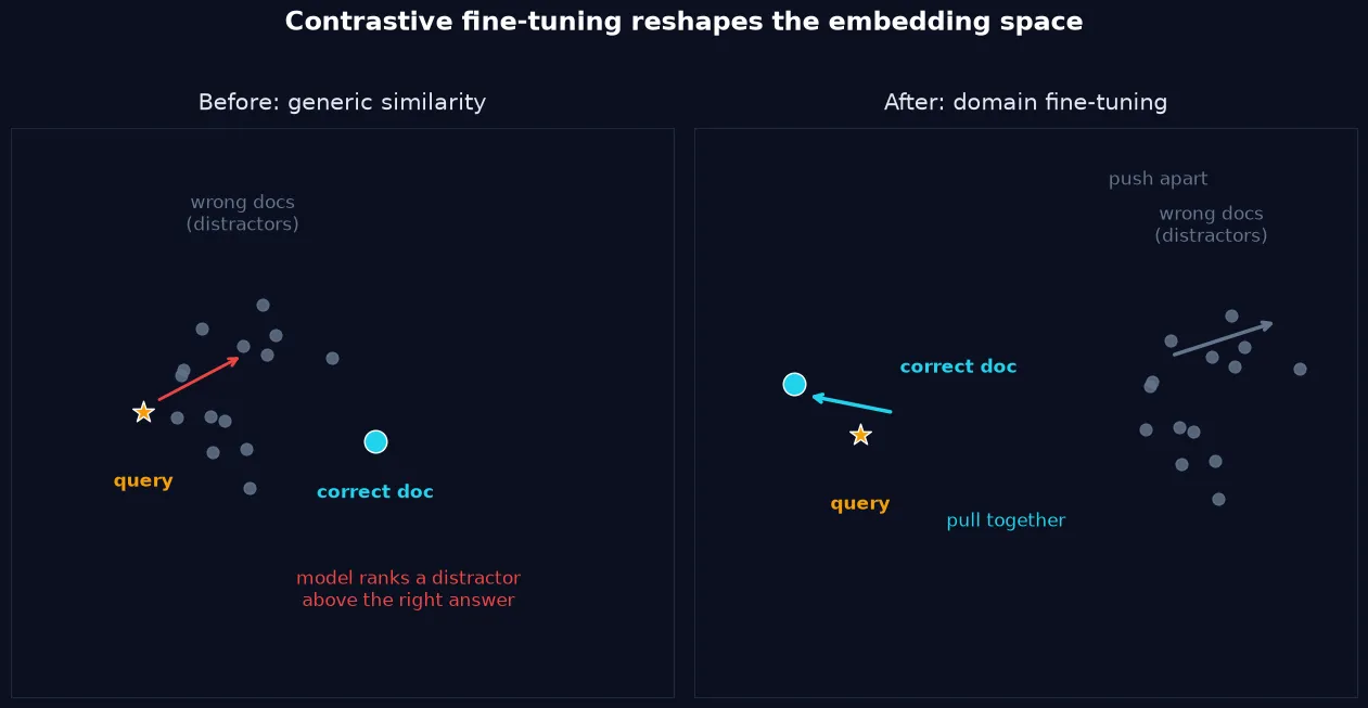
The loss function is the heart of the tutorial. MultipleNegativesRankingLoss works on batches: for each anchor in the batch, its paired positive is the target, and every other positive in the batch serves as a negative. With a batch of 16, each query is contrasted against 1 correct document and 15 wrong ones, for free — no explicit negative mining required. The loss pushes the anchor's embedding toward its positive and away from the 15 in-batch negatives, which is exactly the pull-together/push-apart geometry from the diagram above.
That mechanism dictates one training argument: batch_sampler=BatchSamplers.NO_DUPLICATES. If the same text appeared twice in a batch, it would be treated as both a positive and a negative for the same anchor — a contradiction that poisons the gradient. The no-duplicates sampler prevents it.
from sentence_transformers import (
    SentenceTransformer,
    SentenceTransformerTrainer,
    SentenceTransformerTrainingArguments,
)
from sentence_transformers.sentence_transformer.losses import MultipleNegativesRankingLoss
from sentence_transformers.sentence_transformer.training_args import BatchSamplers

model = SentenceTransformer("sentence-transformers/all-MiniLM-L6-v2")
loss = MultipleNegativesRankingLoss(model)

args = SentenceTransformerTrainingArguments(
    output_dir="models/minilm-3dprint",
    num_train_epochs=4,
    per_device_train_batch_size=16,
    learning_rate=2e-5,
    warmup_steps=0.1,   # float = fraction of total steps used for warmup
    fp16=False,         # CPU training; set True on a CUDA GPU
    bf16=False,
    batch_sampler=BatchSamplers.NO_DUPLICATES,
    logging_steps=5,
    save_strategy="no",
    seed=42,
)

trainer = SentenceTransformerTrainer(
    model=model,
    args=args,
    train_dataset=train_dataset,
    loss=loss,
)
trainer.train()
What each choice does: 4 epochs over 60 pairs at batch size 16 is 16 optimizer steps — tiny, which is the point (more epochs on a small set just memorizes it). A learning rate of 2e-5 is the standard fine-tuning range for these models — large enough to move, small enough not to wreck the pretrained weights. Warmup ramps the learning rate up over the first 10% of steps so the first batches don't yank the weights. fp16=False because this runs on CPU; on a GPU you would flip it to True for speed.
Expected output — the loss should fall steadily across the run:
{'loss': '0.9745', 'grad_norm': '20.86', 'learning_rate': '1.714e-05', 'epoch': '1.25'}
{'loss': '0.4587', 'grad_norm': '6.32', 'learning_rate': '1e-05', 'epoch': '2.5'}
{'loss': '0.4061', 'grad_norm': '12.07', 'learning_rate': '2.857e-06', 'epoch': '3.75'}
{'train_runtime': '78.75', 'train_loss': '0.5946', 'epoch': '4'}
Seventy-nine seconds on a CPU. If your loss does not fall — flat from the first log line — stop: your pairs are probably too easy (the model already ranks them correctly, so there is nothing to learn) or your anchors don't look like real queries. Hard pairs are the fuel; without them the loss has nothing to do.
Step 5: Measure the gain and save the model#
Run the exact same evaluator from step 1 against the trained model — same corpus, same 36 held-out queries:
print(evaluate(model, docs, test_pairs))
model.save_pretrained("models/minilm-3dprint-final")
Expected output:
{'accuracy@1': 0.8611, 'mrr@10': 0.9259}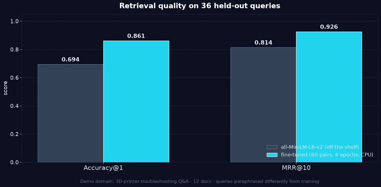
Top-1 accuracy rose from 0.694 to 0.861 — 31 of 36 queries now retrieve the right document first, up from 25. MRR@10 rose from 0.814 to 0.926, meaning even the remaining misses land closer to the top. Six extra correct answers out of 36, from 60 training pairs and 79 seconds of CPU time. That is the entire pitch for fine-tuning embeddings: it is the cheapest large quality gain available in a RAG stack.
A note on honesty: this is a 12-document demo, and small evals are noisy — a swing of one or two queries moves accuracy@1 by three points. The direction and rough magnitude are what transfer to real corpora, not the decimals. On your own data, build a bigger test set (a few hundred queries is the practical minimum) before declaring victory.
Step 6: Ship it — encode once, query forever#
The saved model is a drop-in replacement for the base model everywhere you used it — same 384-dimensional vectors, same interface, just better judgment about your domain. The deployment pattern:
from sentence_transformers import SentenceTransformer

model = SentenceTransformer("models/minilm-3dprint-final")

# Offline, once: embed the corpus and store the vectors
doc_ids = list(docs.keys())
doc_vectors = model.encode(
    [docs[i] for i in doc_ids],
    normalize_embeddings=True,
    show_progress_bar=True,
)
# ... write doc_vectors to your vector DB (Qdrant, pgvector, Pinecone, ...)

# Online, per query: embed the question, take the top-k by cosine similarity
import numpy as np

def retrieve(question, k=3):
    q = model.encode([question], normalize_embeddings=True)
    scores = (q @ doc_vectors.T)[0]
    top = np.argsort(-scores)[:k]
    return [(doc_ids[i], float(scores[i])) for i in top]

print(retrieve("my extruder clicks and nothing comes out mid-print"))
Expected output (document id, cosine similarity):
[('heat_creep', 0.63), ('clogged_nozzle', 0.59), ('under_extrusion', 0.5)]The trap query from step 1 now resolves correctly: heat creep outranks clogged nozzle by a clear margin. That is the behavior you shipped — not a higher benchmark score, but a specific confusion your users actually hit, fixed.
Which approach should you use?#
Fine-tuning is one of four serious ways to fix domain retrieval. Pick by matching the tool to your bottleneck:
- Fine-tune the bi-encoder (this tutorial): best when queries and documents share vocabulary but the model misjudges which shared words matter — domain jargon, product names, internal abbreviations. Cheapest at query time: one embedding, one vector search. Needs 50+ good pairs and a held-out eval.
- Add a cross-encoder reranker: best when the bi-encoder gets the right doc into the top 20 but not to position 1. A reranker reads query and document together (full attention, not two vectors), so it judges finer distinctions — at the cost of running a second model on every candidate at query time.
- Use a bigger/stronger base model: best when you have no training data at all. A stronger off-the-shelf model raises the floor everywhere, but it still doesn't know your jargon, and you pay the latency and memory cost on every query forever.
- Hybrid BM25 + vectors: best when failures are keyword-shaped — part numbers, error codes, exact phrases. BM25 catches the literal matches; vectors catch the paraphrases.
The pragmatic stack, and the one this tutorial composes with: fine-tune the bi-encoder for your domain, keep BM25 alongside it for exact terms, and add a reranker on top only if the top-1 still misses after tuning. Each layer fixes a different failure mode, and each is measurable with the evaluator from step 1.
The takeaway#
Generic embeddings understand language; they don't understand your language. Sixty contrastive pairs — real questions matched to the documents that answer them — teach a small model your domain's notion of similarity in about a minute on a CPU. The recipe that matters: build the held-out eval before you train, make the training pairs as confusable as your real traffic, use in-batch negatives with no duplicate sampler, and trust only the delta between baseline and fine-tuned on queries the model never saw. Do that, and the retriever stops being the part of your RAG pipeline you apologize for.