Differentiable computer vision, batched: hands-on with Kornia 0.9

Most computer vision code is written one image at a time. You load an image with OpenCV, blur it, warp it, detect features in it — and then you write a loop, lose the GPU, and lose the gradients. Kornia exists to remove that loop. It is a library of computer vision operators written as PyTorch ops: they take batches, they take a different parameter per image in the batch, they run on the GPU, and gradients flow through them. kornia/kornia (Apache-2.0) has 12,357 stars and 1,521 forks, and it is back in the conversation because version 0.9.0 shipped on October 23, 2026 — a release the maintainers describe as "more correct, faster, better compile, half-precision, MPS and CUDA" — and the project is now showing up in November's GitHub trending roundups.

The release also sharpens what Kornia is for. The stated direction is to become the reference implementation and executable specification for differentiable computer vision and geometry in the PyTorch ecosystem: explicit conventions, conformance tests, and honest benchmarks over API growth. The README publishes the wins and the losses — batched filters, warps, and feature matching run about 10× to 70× faster than per-image OpenCV or scikit-image on the CPU in the 0.9.0 flagship benchmarks, while on the small overlap with torchvision, eager Kornia is slower and compiled Kornia is faster only for some ops. That candour is the point. This guide installs 0.9.0, runs the operators the README promises, and checks the results against ground truth you can compute yourself.

What you'll need

Python 3.11 or later — Kornia 0.9.0 requires it — and pip. Everything runs on CPU; a GPU speeds up the SIFT step in Step 4 but is not required. No account, no API key, no model download. The versions pinned in this guide: kornia 0.9.0 and torch 2.14.0+cpu, verified on November 8, 2026. Kornia declares a dependency on torch>=2.5.1, so a plain pip install kornia pulls PyTorch too — but that default wheel is the CUDA build, roughly 900 MB. On a CPU-only machine, install the CPU PyTorch first so pip does not fetch the GPU build.

Step 1 — Install Kornia

Install CPU PyTorch, then Kornia 0.9.0:

pip install torch --index-url https://download.pytorch.org/whl/cpu
pip install kornia==0.9.0

If you have a CUDA GPU, skip the first line and run pip install kornia==0.9.0 on its own; pip will bring the CUDA PyTorch build. Verify the install with a smoke test:

python -c "import torch, kornia; print('torch', torch.__version__); print('kornia', kornia.__version__); print('CUDA available:', torch.cuda.is_available())"

Expected output on the CPU-only machine used for this guide:

torch 2.14.0+cpu
kornia 0.9.0
CUDA available: False

Two details matter here. First, pin kornia==0.9.0: the 0.9.0 release is the one this guide verifies, and its API is what the code below uses. Second, the kornia-rs package installs alongside Kornia as a dependency; it provides the Rust-backed image I/O used by the README's quick start. The code in this guide does not need it, but do not be surprised to see it in pip list.

Step 2 — Your first working example: batched transforms with per-sample parameters

The core idea is one line: a Kornia operator takes a batch and a parameter per image. Start with a reproducible test image — a 256×256 textured pattern built from random discs, so nothing needs downloading and every result is deterministic:

import torch

torch.manual_seed(0)

def make_scene(seed=0, h=256, w=256):
    g = torch.Generator().manual_seed(seed)
    img = torch.rand(1, 3, h, w, generator=g) * 0.25
    yy, xx = torch.meshgrid(torch.arange(h), torch.arange(w), indexing="ij")
    for i in range(60):
        cx, cy = int(torch.randint(0, w, (1,), generator=g)), int(torch.randint(0, h, (1,), generator=g))
        r = int(torch.randint(4, 18, (1,), generator=g))
        v = float(torch.rand(1, generator=g))
        m = ((xx - cx) ** 2 + (yy - cy) ** 2) < r * r
        img[0, :, m] = v
    return img

Now blur a four-image batch with a different blur strength per image, and rotate it with a different angle per image. The sigma argument to gaussian_blur2d accepts a (B, 2) tensor; the angle argument to rotate accepts a (B,) tensor. torchvision's functional ops apply one parameter per call; Kornia applies one per sample, in one call:

from kornia.filters import gaussian_blur2d
from kornia.geometry.transform import rotate

batch = make_scene().repeat(4, 1, 1, 1).clone().requires_grad_(True)
sigmas = torch.tensor([[1.0, 1.0], [1.5, 1.5], [2.5, 2.5], [4.0, 4.0]])
blurred = gaussian_blur2d(batch, (9, 9), sigmas)
assert blurred.shape == (4, 3, 256, 256)
blurred.sum().backward()
assert batch.grad is not None and batch.grad.abs().sum() > 0

angles = torch.tensor([0.0, 10.0, -15.0, 30.0])
rot = rotate(batch.detach(), angles)
assert rot.shape == (4, 3, 256, 256)
print("blur ok, grad flows | rotate ok:", tuple(rot.shape))

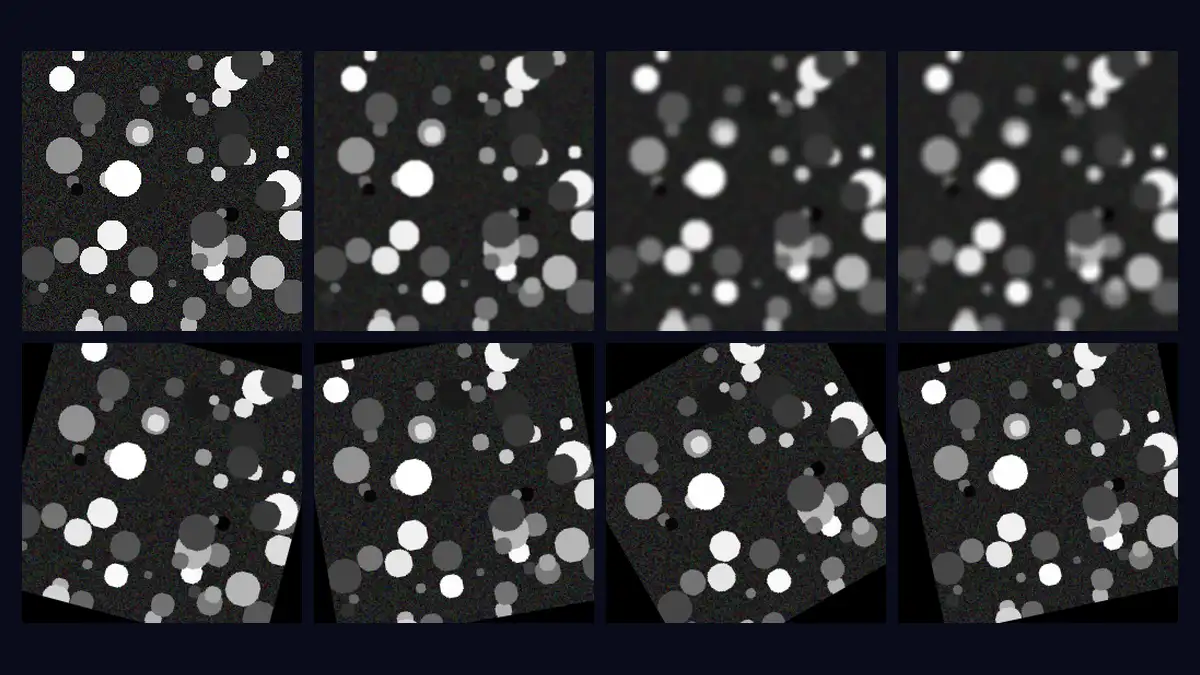
The blur runs in about two seconds on CPU, and the gradient check is the point of the exercise: the blurred output is a differentiable function of the input, so loss.backward() produces a gradient for the input tensor. That is what "differentiable" means here in practice — you can put a blur, a rotation, or a warp inside a training loop or an optimisation, and PyTorch will differentiate through it. The cover image at the top of this article is the same scene under eight of these transforms: three blur strengths, three rotations, and a perspective warp.

Step 3 — Augment an image, its mask, and its keypoints together

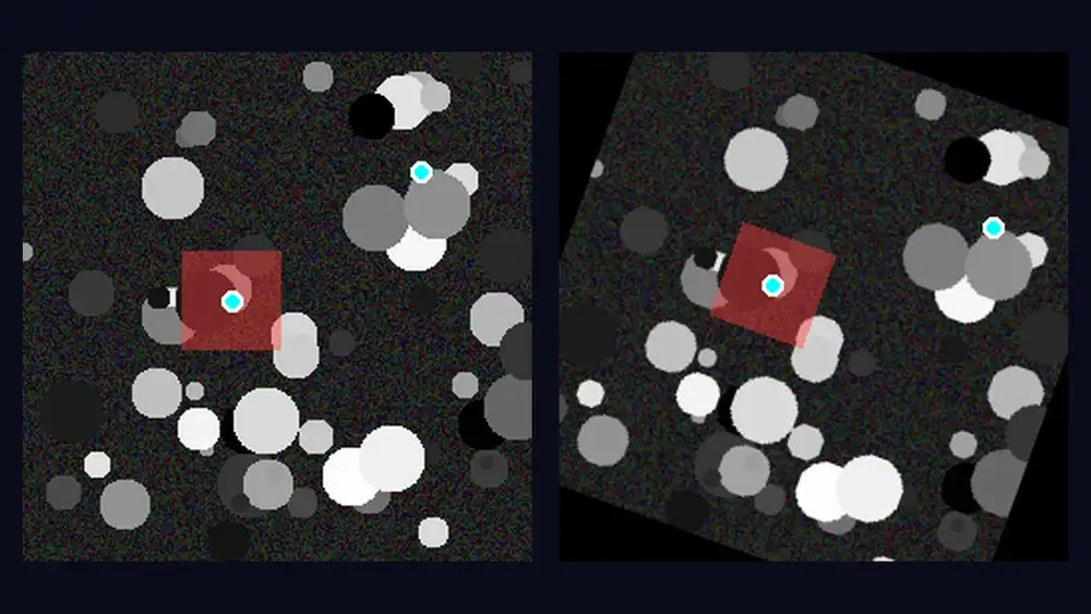
Augmentation breaks training data when the image changes but its labels do not. Kornia's AugmentationSequential applies one sampled transform to the image, the segmentation mask, and the keypoints together, and it can invert the transform afterwards. Build a small annotated example — an image, a rectangular mask, and two keypoints — and rotate all three by a fixed 20 degrees:

from kornia.augmentation import AugmentationSequential, RandomAffine

img = make_scene()
mask = torch.zeros(1, 1, 256, 256)
mask[0, 0, 100:150, 80:130] = 1.0  # rectangle mask
kps = torch.tensor([[[105.0, 125.0], [200.0, 60.0]]])  # (1, 2, 2) x, y

aug = AugmentationSequential(RandomAffine(degrees=(20.0, 20.0), p=1.0),
                             data_keys=["input", "mask", "keypoints"])
out_img, out_mask, out_kps = aug(img, mask, kps)
print("keypoints in :", kps[0].tolist())
print("keypoints out:", [[round(v, 1) for v in p] for p in out_kps[0].tolist()])
print("mask sum in/out:", float(mask.sum()), float(out_mask.sum()))
print("mask unique vals:", torch.unique(out_mask.round()).tolist())

Expected output:

keypoints in : [[105.0, 125.0], [200.0, 60.0]]
keypoints out: [[107.2, 117.5], [218.7, 88.9]]
mask sum in/out: 2500.0 2498.0
mask unique vals: [0.0, 1.0]

Three checks pass. The keypoints moved with the image: (105, 125) is now (107.2, 117.5) and (200, 60) is now (218.7, 88.9). The mask kept its area — 2,500 pixels in, 2,498 out, the two-pixel difference being interpolation at the rotated edges — and it stayed binary, with only 0.0 and 1.0 as values, so it is still a usable segmentation mask rather than a smeared probability map. The degrees argument is a range, so (20.0, 20.0) pins the rotation to exactly 20 degrees; in real training you would pass a range like (-30.0, 30.0) and let each batch sample its own angle. Finally, invert the transform and confirm the round trip:

back_img, back_mask, back_kps = aug.inverse(out_img, out_mask, out_kps)
print("inverse round-trip mean abs err:", round(float((back_img - img).abs().mean()), 4))

Expected output: inverse round-trip mean abs err: 0.0458. The error is not zero because the forward pass resamples with bilinear interpolation, and interpolation loses information — but a mean absolute error of 0.046 on a 0–1 image is a faithful inversion, and it is the number to expect if you reproduce this step.

Step 4 — A real end-to-end use case: match two views and recover the homography

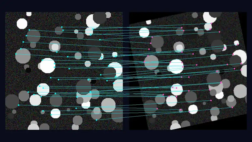
Transforms and augmentation are the warm-up. The use case that shows what Kornia is for is geometric: take two views of the same scene, find the features they share, and recover the geometric transform between them. That is the core step of image stitching, registration, and visual localisation. Build a second view by warping the scene with a known homography — a 12-degree rotation about the centre, a 0.95 scale, and a (10, −6) translation — so the answer is known before the estimation starts:

from kornia.feature import SIFTFeature, match_snn
from kornia.geometry.ransac import RANSAC
from kornia.geometry.transform import warp_perspective, get_rotation_matrix2d
from kornia.color import rgb_to_grayscale

scene = make_scene(seed=7)
M = get_rotation_matrix2d(torch.tensor([[127.5, 127.5]]),
                          torch.tensor([12.0]), torch.tensor([[0.95, 0.95]]))
H = torch.eye(3).unsqueeze(0)
H[0, :2, :] = M[0]
H[0, 0, 2] += 10.0
H[0, 1, 2] += -6.0
view2 = warp_perspective(scene, H, (256, 256))

Two notes on that block. get_rotation_matrix2d takes the centre as a (B, 2) tensor, the angle as (B,), and the scale as a (B, 2) tensor — passing a one-element scale tensor raises a ValueError, which is the single sharpest edge in this API. And the homography is built by writing the 2×3 rotation matrix into a 3×3 identity and adding the translation to its last column.

Now detect SIFT features in both views, match their descriptors, and estimate the homography with RANSAC:

sift = SIFTFeature(num_features=2000)
lafs1, _, desc1 = sift(rgb_to_grayscale(scene))
lafs2, _, desc2 = sift(rgb_to_grayscale(view2))
dists, idxs = match_snn(desc1[0], desc2[0], 0.8)
kp1 = lafs1[0, idxs[:, 0], :, 2]  # matched keypoints, view 1 (N, 2) x, y
kp2 = lafs2[0, idxs[:, 1], :, 2]  # matched keypoints, view 2

ransac = RANSAC(model_type="homography", inl_th=2.0, max_iter=1000, confidence=0.999)
H_est, inliers = ransac(kp1, kp2)
print("matches:", len(idxs), "| inliers:", int(inliers.sum()))

Expected output on CPU: 2,000 features per view in about 13 seconds, then matches: 223 | inliers: 192. The local affine frames returned by SIFTFeature are (B, N, 2, 3) tensors, and the keypoint centre is the last column — lafs[..., :, 2] — which is the indexing to remember. match_snn applies Lowe's ratio test at the 0.8 threshold: a match survives only if its nearest neighbour is clearly closer than its second-nearest. RANSAC then fits the homography to the surviving correspondences with a 2-pixel inlier threshold.

The check that matters is the comparison against the known homography. Normalise both matrices by their bottom-right element and reproject the inlier keypoints through each:

def norm(Hm):
    return Hm / Hm[2, 2]

err_H = float((norm(H_est) - norm(H[0])).abs().mean())
ones = torch.ones(int(inliers.sum()), 1)
p1h = torch.cat([kp1[inliers], ones], dim=1)
proj_true = (H[0] @ p1h.T).T
proj_true = proj_true[:, :2] / proj_true[:, 2:3]
proj_est = (H_est @ p1h.T).T
proj_est = proj_est[:, :2] / proj_est[:, 2:3]
reproj = float(((proj_true - proj_est) ** 2).sum(1).sqrt().mean().detach())
print("H mean abs diff:", round(err_H, 4), "| mean reproj err (px):", round(reproj, 3))

Expected output: H mean abs diff: 0.003 | mean reproj err (px): 0.059. The estimated homography differs from the ground truth by 0.003 on average, and reprojecting the inliers through the two matrices disagrees by six hundredths of a pixel. That is a correct answer, not an approximate one — and it was computed from the images alone, with no access to the homography used to build the second view.

Step 5 — Sanity-check image quality with SSIM and PSNR

Once images are tensors, their quality metrics are tensor ops too. Score the σ=1 blurred image from Step 2 against the original with kornia.metrics:

from kornia.metrics import ssim, psnr

orig0 = batch.detach()[0:1]
s = float(ssim(orig0, blurred[0:1], window_size=11).mean().detach())
p = float(psnr(orig0, blurred[0:1], max_val=1.0).detach())
print("ssim(orig, blurred sigma=1):", round(s, 4), "| psnr:", round(p, 2))

Expected output: ssim(orig, blurred sigma=1): 0.5512 | psnr: 22.97. The SSIM looks low for a light blur, and the reason is the test image: it is deliberately high-frequency — random discs on noise — so even a σ=1 blur changes a large share of its structure. Expect a higher SSIM for the same blur on a smoother natural photo. The numbers are useful as a regression check all the same: put them in a test, and a future change to your pipeline that moves them has to explain itself.

When to use this vs alternatives

Versus torchvision. torchvision covers the common ops — resizing, cropping, flipping, colour jitter, blur — and Kornia's own benchmarks say that on that small overlap, eager Kornia is slower on the same GPU, while compiled Kornia is faster for hue, colour jitter, and Gaussian blur. Choose Kornia when you need what torchvision does not have: 1,200+ operators, per-sample parameters in one batched call, camera models and epipolar geometry, batched minimal solvers and RANSAC, and feature detection and matching on the GPU.

Versus OpenCV. OpenCV wins single-image uint8 CPU work — Kornia's README says so outright. OpenCV is the right call for a classic pipeline that processes one frame at a time on CPU and never needs a gradient. Choose Kornia when the work is batched, when it runs on the GPU, or when a transform or a loss has to be differentiable.

Versus Albumentations. Albumentations is fast, CPU-first, and excellent at augmentation alone, with a large catalogue of transforms. It is not differentiable and it does not do geometry estimation or feature matching. Use it for augmentation-only pipelines; use Kornia when the same library has to augment, estimate geometry, and feed a training loop.

Versus raw PyTorch. For a single fixed-parameter operation — one blur, one resize — a few lines of PyTorch or torchvision are just as good, and Kornia's README says so. Kornia pays off where a hand-written version gets long or fragile: per-sample parameters, annotation-consistent augmentation, solvers, and matching.

When not to use it. Skip Kornia for a single fixed op, for a uint8 single-image CPU pipeline, and for half-precision work on CPU without checking the precision guide first: the 0.9.0 README records 239 float16 and 251 bfloat16 known-failure entries in its CPU manifests, mostly in augmentation and geometry, so float32 is the safe default on CPU. And if your whole pipeline is already OpenCV and never touches a tensor, adding Kornia adds a dependency for nothing.

The takeaway

Kornia 0.9.0 is a library that treats computer vision as tensor computation: batches instead of loops, a parameter per image instead of one per call, gradients through blurs and warps, and geometry — SIFT matching, RANSAC, homographies — in the same library as the filters. Install it with two pip commands, prove the loop with a batched blur and a gradient check, keep your masks and keypoints in sync with one augmentation call, and recover a homography from two views to sub-tenth-pixel accuracy. The whole verified path runs in about half an hour on CPU, costs nothing, and leaves you with operators you can drop into a training loop instead of a script that processes one image at a time.

Sources

• kornia/kornia on GitHub — repository, README, install instructions, and 0.9.0 release notes
• kornia on PyPI — version 0.9.0, dependencies, and Python requirement
• Kornia docs — API reference, performance page, and precision guide
• kornia.org — tutorials and examples