Your 32K context window is a marketing number: measure what your model actually remembers
Vendors advertise 128K, 200K, million-token context windows — but how much of that window does a model actually use? Build the classic needle-in-a-haystack test, run it on a local model, and read the heatmap like an eval engineer.

Every major model release this year has advertised a bigger context window — 128K, 200K, a million tokens and beyond. The number on the box keeps growing, and it is tempting to treat it as a capability: stuff the whole codebase, the whole inbox, the whole document archive into the prompt and let the model sort it out.
That number is a capacity, not a capability. What matters for your application is effective context: how much of the window the model actually uses when the fact you need sits 40,000 tokens deep. Those two numbers are not the same, and the gap between them has been measured repeatedly since late 2023. The uncomfortable part is that nobody will measure it for your model, your prompt shape, your task — the effective context of a small local model answering terse questions looks nothing like the effective context of a frontier model doing multi-hop reasoning.
This tutorial fixes that. You will build the classic needle-in-a-haystack test from scratch, run it against a real model on your own machine, and read the resulting heatmap the way eval engineers do. No API keys, no GPU, about twenty minutes of compute. When you finish, you will know exactly how far you can trust your setup — and what to do when the answer is "not as far as the brochure says."
The test in sixty seconds#
The method comes from Greg Kamradt's November 2023 pressure test of GPT-4 and Claude 2.1, and it has barely changed since because the core idea is airtight:
- Plant a needle — one short, distinctive fact — inside a large body of filler text (the haystack) at a controlled depth: 10% of the way in, 50%, 90%.
- Ask the model to retrieve it, with the haystack as context.
- Sweep two axes — total context length and needle depth — and score each cell pass/fail.
- Render the grid as a heatmap. Green where the model remembers, red where it forgets.
Kamradt's headline finding still frames the whole field: at the largest context lengths, neither GPT-4 (128K) nor Claude 2.1 (200K) reliably retrieved a planted fact, and recall degraded non-uniformly with depth. A few months later, Liu et al.'s Lost in the Middle (2023) gave the phenomenon its name and its shape: accuracy follows a U-shaped curve — best when the needed information sits at the very beginning or the very end of the context, worst in the middle — even in models explicitly built for long contexts. In one of their setups, GPT-3.5-Turbo with the answer buried mid-context scored below its own closed-book accuracy: the extra context actively hurt.
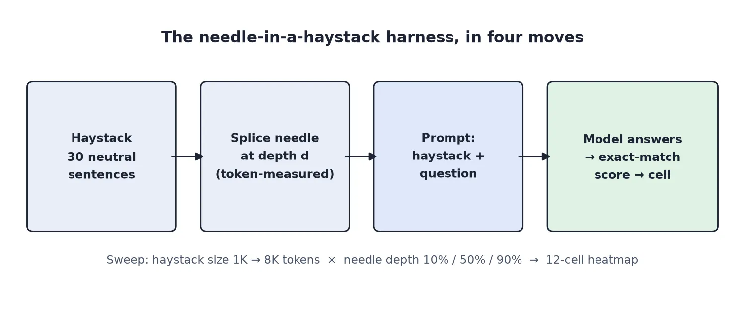
Your heatmap is a compressed version of the same experiment, calibrated to your model. Here is what the machinery looks like:
What you'll need#
- Python 3.10+ and pip. Everything runs on CPU.
- ~1.2 GB of disk for the model weights. No GPU, no API key, no account anywhere.
- PyTorch (CPU build) + Hugging Face Transformers — the standard local-inference stack, installed from prebuilt wheels.
- A small instruction-tuned model: Qwen2.5-0.5B-Instruct (~1 GB). Half a billion parameters is deliberately modest: it keeps the full sweep under an hour on a laptop CPU, and the shape of the result — where performance breaks — is what you are after, not the absolute scores.
python3 -m venv needle && source needle/bin/activate
pip install torch --index-url https://download.pytorch.org/whl/cpu
pip install transformers matplotlib huggingface_hub
# ~1 GB download — Qwen2.5-0.5B-Instruct weights
# (huggingface-cli is deprecated in huggingface_hub 5.x; use hf)
hf download Qwen/Qwen2.5-0.5B-Instruct --local-dir ./qwen2.5-0.5b
Two notes before you start. First, the model is small on purpose, and small models forget sooner — treat your absolute numbers as a floor for your setup, not as a verdict on the technique. Second, this is a demonstration grid (one trial per cell); a production eval would run multiple trials per cell and average, exactly as Kamradt's original did. The harness below is structured so you can add that in one line.
Step 1: Plant a needle, build a haystack#
The haystack must be boring and uniform — if the filler is too distinctive, the model can cheat by pattern-matching instead of retrieving. Thirty neutral sentences about harbor logistics, shuffled and repeated, work well. The needle is one sentence that could not be guessed:
NEEDLE = "The access code for the Harbor Street warehouse is 847291."

FILLER = [
    "The harbor district wakes early, with gulls circling above the container ships.",
    "Maritime law requires every vessel to log its cargo before entering the port.",
    "The old lighthouse was converted into a museum in the late nineteen hundreds.",
    "Tide charts are published quarterly by the coastal survey office.",
    "A shipment of machine parts arrived on the morning ferry from the mainland.",
    "The warehouse district spans fourteen blocks along the northern waterfront.",
    "Customs officers inspect roughly one in every twelve incoming containers.",
    "The ferry schedule changes twice a year, in spring and in autumn.",
    "Local fishermen report that the salmon run arrived two weeks early this year.",
    "The port authority approved funding for three new docking cranes.",
    "Fog is most common in the harbor during the early autumn months.",
    "The maritime museum hosts guided tours every Saturday afternoon.",
    "Shipping insurance rates rose slightly after last winter's storms.",
    "The coastal railway connects the port to five inland distribution centers.",
    "A new cold-storage facility opened near the southern pier last spring.",
    "Harbor pilots board incoming vessels about two miles offshore.",
    "The annual regatta draws sailing crews from across the region.",
    "Dockworkers begin their shifts an hour before the first tide change.",
    "The lighthouse keeper's logbook dates back over a hundred years.",
    "Seagulls follow the fishing boats back into the harbor each evening.",
    "The port's container yard can hold up to eight thousand steel boxes.",
    "A tugboat escorts every large tanker through the narrow channel.",
    "The fish market opens to wholesalers well before sunrise.",
    "Coastal erosion studies are conducted along the cliffs every summer.",
    "The harbor master keeps a detailed record of every vessel movement.",
    "Storm shutters are tested on all waterfront buildings each October.",
    "The old cannery building now houses artists' studios and a cafe.",
    "Buoys mark the safe channel for ships entering the bay.",
    "The maritime academy graduates about two hundred cadets per year.",
    "Night ferries run on a reduced schedule during the winter months.",
]
The critical detail is depth control in tokens, not sentences. "Halfway through the document" must mean half the tokens, because the model's context window is measured in tokens and attention dilutes per token. Tokenize the filler, cut it at the target length, and splice the needle in at the requested fraction:
import torch
from transformers import AutoModelForCausalLM, AutoTokenizer

torch.set_num_threads(4)
tokenizer = AutoTokenizer.from_pretrained("./qwen2.5-0.5b")
model = AutoModelForCausalLM.from_pretrained("./qwen2.5-0.5b",
                                            torch_dtype=torch.float32)
model.eval()

def build_haystack(target_tokens, depth_frac, rng):
    filler_ids = []
    order = FILLER[:]
    rng.shuffle(order)
    i = 0
    while len(filler_ids) < target_tokens:
        filler_ids.extend(tokenizer.encode("
" + order[i % len(order)],
                                           add_special_tokens=False))
        i += 1
    filler_ids = filler_ids[:target_tokens]
    needle_ids = tokenizer.encode(NEEDLE, add_special_tokens=False)
    split = int(len(filler_ids) * depth_frac)
    ids = filler_ids[:split] + needle_ids + filler_ids[split:]
    text = tokenizer.decode(ids)
    assert text.count(NEEDLE) == 1, "needle splice failed"
    return text
Verify the splice the paranoid way: after building each haystack, assert the needle string is present exactly once. A needle that got truncated by your token budget invalidates the cell silently — this is the most common bug in DIY harnesses.
Step 2: Ask one question, score it ruthlessly#
Ask the retrieval question with the haystack as context, then score with the strictest check available: does the response contain the exact code? No LLM judge, no partial credit — binary scoring is what makes the heatmap honest.
QUESTION = ("What is the access code for the Harbor Street warehouse? "
            "Reply with only the code, nothing else.")

@torch.inference_mode()
def ask(haystack):
    prompt = tokenizer.apply_chat_template(
        [{"role": "user",
          "content": f"Read the following document carefully.

{haystack}

Question: {QUESTION}"}],
        tokenize=False, add_generation_prompt=True)
    inputs = tokenizer(prompt, return_tensors="pt")
    out = model.generate(**inputs, max_new_tokens=24, do_sample=False,
                         pad_token_id=tokenizer.eos_token_id)
    new_tokens = out[0][inputs["input_ids"].shape[1]:]
    return tokenizer.decode(new_tokens, skip_special_tokens=True).strip()

answer = ask(haystack)
correct = "847291" in answer
Three choices here are load-bearing. do_sample=False (greedy decoding) removes sampling noise so the grid measures the model, not the dice. max_new_tokens=24 keeps generations short — prefill dominates the runtime, and a six-digit answer needs no more. And the question goes after the document, matching how retrieval prompts work in practice (and matching Kamradt's original setup).
Step 3: Run the grid#
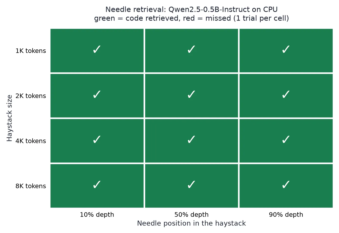
Now sweep both axes. Four context lengths (1K, 2K, 4K, 8K tokens) against three depths (10%, 50%, 90%) gives twelve cells — enough to see the shape of the failure without burning an afternoon:
import random, time, json

results = []
for length in [1000, 2000, 4000, 8000]:
    for depth in [0.10, 0.50, 0.90]:
        haystack = build_haystack(length, depth, random.Random(42))
        t = time.time()
        answer = ask(haystack)
        results.append({"tokens": length, "depth": depth,
                        "correct": "847291" in answer,
                        "answer": answer, "seconds": round(time.time() - t, 1)})
json.dump(results, open("results.json", "w"), indent=2)
On a 2-thread CPU this took about 53 minutes for all twelve cells — the cost is almost entirely prefill (reading the haystack), which is why short max_tokens matters. Here is the heatmap from that run:
Step 4: Read the heatmap like an eval engineer#
Here is the honest read of this particular heatmap: it is all green. Qwen2.5-0.5B-Instruct retrieved the code in all twelve cells — every length from 1K to 8K tokens, the needle at 10%, 50%, and 90% depth. No rightward fade, no middle dip, no cliff. That is a real measurement, and it tells you something useful: for this task shape — one distinctive, high-signal fact, greedy decoding, a terse question — this model stays reliable through 8K tokens. But notice what it does not tell you. The sweep stopped at 8K, a quarter of the model's advertised 32K window, and a single code buried in neutral filler is the easiest long-context task there is; multi-hop reasoning over diffuse evidence breaks much earlier. So the all-green grid is not a verdict that the full 32K is usable — it is the baseline against which you push the length axis further (16K, 32K) and add more trials per cell until red appears. The value of the harness is not the colors you got; it is that you now own the instrument that finds where your setup turns red.
Three patterns to check for in any heatmap, yours included:
- The rightward fade. Accuracy decays as context grows, even at fixed depth. This is context rot: every extra thousand tokens of filler steals a little attention from the needle. If your application's "long" prompts sit in the faded zone, you are paying for context that hurts.
- The middle dip. At a fixed length, the 50%-depth cell underperforms the 10% and 90% cells — the U-shape from Lost in the Middle. The mechanism is structural: attention sinks and positional encodings privilege the start and end of a sequence, so the middle is where facts go to be forgotten.
- The cliff. A sharp vertical boundary where everything past some length fails regardless of depth. That is your model's effective context for this task shape — write it down, because it is almost certainly smaller than the number on the model card.
One caution from the literature before you generalize: the U-shape is well established for single-pass factual retrieval, but it is not a law of physics. Follow-up work has found it weaker or absent in some newer models on some task shapes, attributing the difference to better positional encodings and training curricula. Your heatmap measures your model on your task — which is exactly why running it beats citing a paper.
What to do when the number disappoints you#
A disappointing heatmap is not a dead end; it is a design input. Four mitigations, in order of effort:
- Put critical facts at the edges. The cheapest fix in existence: place the instruction and the must-remember facts at the very start or the very end of the prompt. If both matter, state them twice — once up top, once at the bottom. You are designing around the U-shape instead of fighting it.
- Retrieve, don't stuff. Liu et al. found that retriever recall keeps climbing as you add documents while reader accuracy saturates early — past a point, each extra retrieved chunk is pure noise tax. A tight top-k (3–5 chunks) into a short prompt routinely beats dumping fifty chunks into a long one, and it is cheaper twice over: fewer input tokens, better accuracy.
- Keep the haystack lean on purpose. Kamradt's own conclusion from the original test: less context means more accuracy. Strip boilerplate, dedupe repeated content, and summarize what the model only needs approximately. Every token you cut is attention returned to the tokens that matter.
- Make the model show its receipt. Ask for the answer plus a quote of the supporting span. A model that can quote the needle verbatim is far less likely to be hallucinating than one that blurts a plausible-looking code — and when it quotes the wrong span, you have a precise debugging signal instead of a mystery.
Which approach should you use?#
The heatmap tells you where your model stops being reliable. What you build on top depends on where your workload sits relative to that boundary:
| Your situation | Use | Why |
|---|---|---|
| Everything you need fits inside the green zone | Stuff it in the prompt, facts at the edges | Simplest architecture; no retrieval infra to maintain |
| Corpus is 10–100× the green zone | RAG with tight top-k (3–5 chunks) | Reader accuracy saturates early — extra chunks are noise tax |
| You need many facts from across a long document | Map-reduce over chunks, then synthesize | Each chunk is read in its own green-zone pass; the middle dip never triggers |
| Facts must be found and reasoned over jointly | Agentic retrieval (search tools + iterative reads) | The agent re-queries instead of holding everything at once |
The through-line: never design a system that requires the model to reliably use its red zone. The brochure number is for marketing; the heatmap number is for architecture.
The takeaway#
Context windows are cheap to advertise and expensive to trust. In about twenty minutes, with no GPU and no API key, you measured the gap between the two for a real model: where retrieval holds, where the middle dip bites, and where the cliff drops off. That measurement — a twelve-cell grid and an honest heatmap — is worth more than any model card, because model cards describe capacity and your application lives or dies on effective use.
Run the harness again whenever something changes: a new model, a new quant, a new prompt shape, a longer document type. The grid is the same; only the colors move. And the next time someone proposes "just put the whole thing in context," you will have a picture that answers the question before the debate starts.