Speed up your local LLM server: hands-on with inference-optimisation-skill
inference-optimisation went from zero to 1,272 stars in four days by replacing local-LLM tuning folklore with a method: compute the ceiling first, change one thing at a time, and let interleaved controls decide what counts as a win. This tutorial runs the whole loop on a real server — and reports the two levers that failed.
- The project: sybil-solutions/inference-optimisation-skill, 1,272 stars, MIT, created November 16, 2026 — the most-starred new AI project of the week, 588 stars in its first day. Standard-library Python plus bash; works with vLLM, SGLang, llama.cpp, ExLlama, MLX, and TensorRT-LLM.
- The method: ceiling first, one change per experiment, controls on both sides, medians of 6+ samples, accept only if it beats both neighbouring controls and regresses nothing by more than ~3%. Log every result, including failures.
- Verified here: Qwen3-1.7B-Q4_K_M on a 4-vCPU shared VM: decode ceiling 12-16 tok/s (1.342 GB per token at 15.8-21.3 GB/s); baseline decode 10.4-14.0 tok/s across three controls; prefill 19-23 tok/s at ~1,136 tokens.
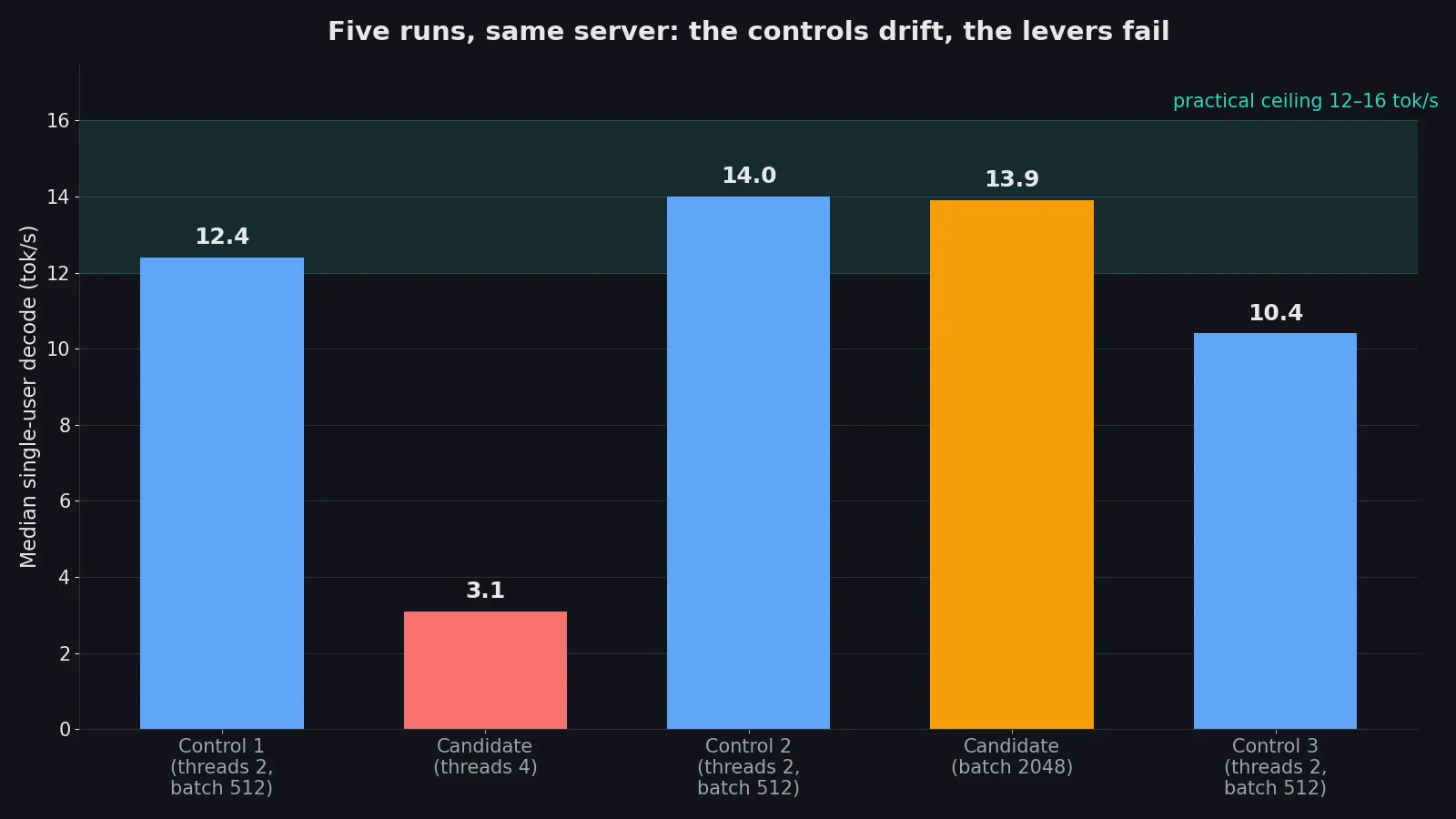
- Lever 1 — threads 2 to 4: REJECTED. Decode collapsed 12.4 to 3.1 tok/s (-75%) while prefill rose 19 to 22. Oversubscription on ~1.5 shared cores; fails the no-regression rule by a factor of four.
- Lever 2 — batch 512 to 2,048: REJECTED, no effect. Decode 13.9 vs controls of 14.0 and 10.4; prefill 19 vs 23 and 19. Beats neither neighbouring control on its target metric. Best config is the baseline; needle gate failed 0/3 (base model, see Step 7).

Most local-LLM tuning advice is a list of flags. Raise the batch size, turn on the graph cache, try a draft model — and if the number goes up, call it a win. The problem is that on a shared machine the number goes up and down by itself. The same configuration measured 53.8 tokens per second and then 49.5 an hour later, with nothing changed. A single-run "win" is usually drift wearing a costume.
inference-optimisation (sybil-solutions/inference-optimisation-skill) is an agent skill that replaces the flag list with a method. It was created on November 16, 2026, and by November 20 it had 1,272 stars — the most-starred new AI project of the week — after picking up 588 stars in its first day. It is MIT-licensed, written in standard-library Python and bash, and it works with any engine: vLLM, SGLang, llama.cpp, ExLlama, MLX, TensorRT-LLM. The method is six rules long: compute the theoretical ceiling first; change one thing at a time; measure every change against interleaved controls; take medians, never best runs; log every result including the failures; and prove full-context stability before calling anything best.
This tutorial runs the whole loop on a real server and reports what actually happened — including the two levers that failed. You will install the skill, measure your hardware, compute the ceiling for a 1.7-billion-parameter model, take a baseline, test a thread-count change and a batch-size change with controls on both sides, and end with a qualified best configuration. No API key, no account, no GPU. Every number below was measured in this run, on a small shared virtual machine, with the harness described in the verification section.
What you will need#
- Python 3.10 or newer. The skill's harness is standard-library Python plus bash, so there is nothing to install for the skill itself. This tutorial used Python 3.12.3.
- A local model server with an OpenAI-compatible API. Any engine works. This tutorial used the
llama-cpp-python0.3.35 server and Qwen3-1.7B-Q4_K_M (Unsloth's quantisation, 1.1 GB), served on port 8080 with a 4,096-token context. vLLM and SGLang users point the same harness at their own server; nothing in the loop is llama.cpp-specific. - A model file. Any GGUF, EXL2/EXL3, AWQ, GPTQ, FP8, or MLX model the skill's ceiling math can describe. The demo model is 1.7 billion parameters, so it runs on a CPU-only machine.
- About 30 minutes and roughly 1.5 GB of disk for the model and the Python packages. No multi-gigabyte downloads are needed anywhere in this tutorial.
- No account and no API key. Everything runs locally. A coding agent (Claude Code or any agent that loads
SKILL.md-style skills) is optional: the skill can drive the loop for you, but every command in this tutorial is run by hand, and the skill also ships aPROMPT.mdfor agents that do not load skills.
Step 1: Install the skill#
Clone the repository and copy the skill into your agent's skills folder. For Claude Code the install is user-level:
git clone https://github.com/sybil-solutions/inference-optimisation-skill
mkdir -p ~/.claude/skills
cp -r inference-optimisation-skill/skills/inference-optimisation ~/.claude/skills/
Other agents point at skills/inference-optimisation/SKILL.md directly, or paste PROMPT.md as the task prompt. The skill has three parts. SKILL.md is the procedure: inventory, ceilings, ground rules, the loop, and lever order. The references/ folder is loaded only when needed and covers ceiling maths with a worked example, measurement traps, levers tagged general or stack-specific, known engine and hardware gotchas, and the publishing rules. The scripts/ folder is the harness: bench.py benchmarks any OpenAI-compatible server, ceiling.py computes theoretical maxima from measured hardware, queue.sh serialises interleaved runs, and mem.sh reports real memory footprint including driver residency on unified-memory GPUs.
The no-agent quick start, straight from the README, is four commands:
S=skills/inference-optimisation
python3 $S/scripts/ceiling.py $S/examples/ceiling-ornith-b390.json        # ceilings
mkdir -p configs && cp $S/examples/config-existing-server.json configs/base.json   # edit base_url/model
python3 $S/scripts/bench.py run configs/base.json --long 131072            # one run
bash $S/scripts/queue.sh base cand base                                     # interleaved A/B
python3 $S/scripts/bench.py show                                            # ledger table
Before you touch anything, the skill wants a working directory with four things: PLAN.md (a timestamped log of every experiment, with numbers, verdict, and reason), THEORY.md (the ceilings), ledger.jsonl (one line per run, from the harness), and configs/ (one JSON per run). Create them now; the rest of the tutorial fills them in.
Step 2: Measure the hardware, don't trust the spec sheet#
Every ceiling in the next step divides by a measured number, so measure first. Two measurements matter: real memory bandwidth (a device-to-device copy of a large buffer) and real matmul throughput (a large square GEMM). Spec sheets quote peak figures your machine never reaches under a real workload.
The machine used here is a small shared virtual machine: 4 vCPUs (about 1.5 cores of shared capacity), 7.9 GB of RAM, no GPU. Copying a 1 GB buffer in memory measured 42.6 GB/s counting read plus write traffic, and a pure-read pass measured 15.8 GB/s. The two probes bracket the true read bandwidth: the copy's read share is about 21 GB/s, the pure-read pass 15.8 GB/s. That range matters in the next step, because the ceiling inherits its width.
Record the state of the machine too: power source, performance profile, and anything else running. A laptop on battery runs 8–10% slower, and the skill's harness refuses to run unless the machine is plugged in and idle. On a shared VM the equivalent rule is to note the load average with every run, because another tenant's job is your battery.
Step 3: Compute the ceiling before you optimise anything#
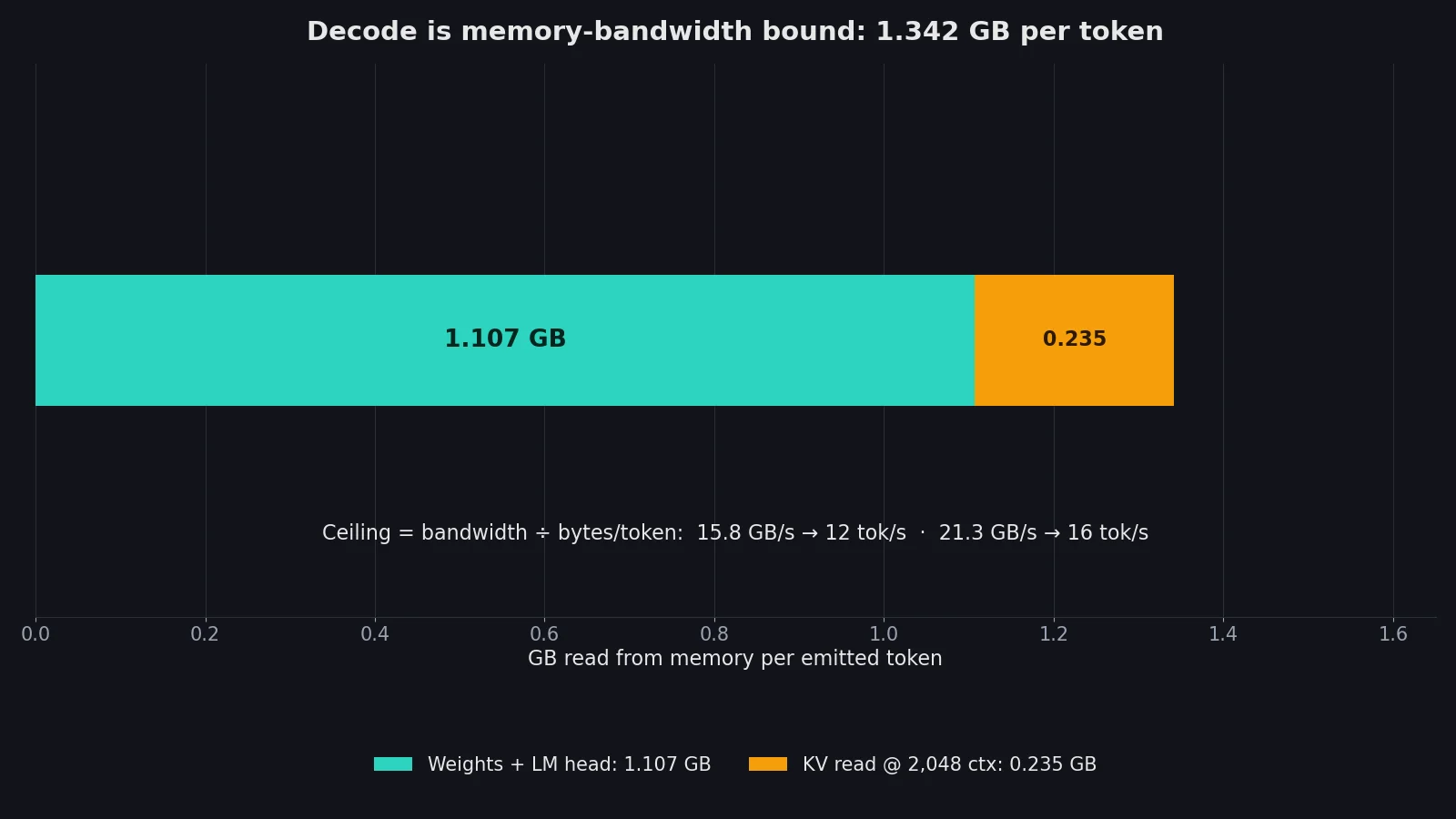
This is the step that makes the whole method worth using. Decode is memory-bandwidth bound: each emitted token forces the server to read the weights, the LM head, and the KV cache for the working context. Count those bytes, divide by measured bandwidth, and you have the fastest decode that physics allows on your machine. Prefill is compute bound instead: about 2 FLOPs per active parameter per token, divided by roughly half of measured peak FLOPs.
For the demo model, Qwen3-1.7B in Q4_K_M, the arithmetic is:
- Weights and LM head: the model file is 1,107,409,472 bytes — about 1.107 GB — and that is the dense weights plus the LM head together, already quantised.
- KV cache per token: 28 layers × 2 (key and value) × 8 KV heads × 128 head dimension × 2 bytes (FP16 cache) = 114,688 bytes per token. At a 2,048-token working context that is 0.235 GB read per emitted token.
- Total bytes per token: 1.107 + 0.235 = 1.342 GB.
- Decode ceiling: 15.8 GB/s ÷ 1.342 GB/token ≈ 12 tok/s at the low bandwidth estimate, and 21.3 GB/s ÷ 1.342 ≈ 16 tok/s at the high one. The ceiling is 12–16 tok/s, and the width is honest: it comes from the two bandwidth probes disagreeing.
Write that into THEORY.md before you measure anything. The point is not the number itself; it is what the number does to your expectations. If someone promises you 100 tok/s from this model on this box, the ceiling says no in one line. The skill's own worked example makes the same point on bigger hardware: an Ornith 35-billion-parameter MoE on an Intel Arc B390 laptop iGPU had a no-speculation decode ceiling of 68 tok/s, and the team reached 53 — about 55% of it, with the rest lost to quantised kernel efficiency. Report progress as a percentage of the practical ceiling, never as a bare number.
Step 4: Measure the baseline, with medians and a warmup#
Start the server with a plain, defensible configuration and measure it the way the skill demands: a discarded warmup run (cold first runs are not representative), then at least six decode samples, median — never the best run. Count tokens from the server's usage stats, never from streamed chunks: with speculative decoding, engines emit several tokens per chunk, and counting chunks under-reports. Size prompts with the real tokenizer. Build prompts before the clock starts, make them unique per run so prefix caching cannot hit, and keep the prompt panel fixed across configs, because acceptance and speed both depend on prompt content.
The baseline launch used here:
python3 -m llama_cpp.server \
  --model Qwen3-1.7B-Q4_K_M.gguf --model_alias qwen3-1.7b \
  --host 127.0.0.1 --port 8080 \
  --n_ctx 4096 --n_batch 512 --n_ubatch 512 --n_threads 2
Two threads, the default 512-token batch, a 4,096-token context. The decode probe was a fixed prose prompt continued for 64 tokens, greedy, six samples. The prefill probe was a cold, unique ~1,136-token prompt (1,024 words, calibrated at 1.1 tokens per word against the server's own tokenizer), three samples, measured as prompt tokens divided by time to first token.
The baseline, measured three times across the run as interleaved controls, was:
| Run | Decode, 1 user (median of 6) | Prefill at ~1,136 tokens (median of 3) |
|---|---|---|
| Control 1 | 12.4 tok/s | 19 tok/s |
| Control 2 | 14.0 tok/s | 23 tok/s |
| Control 3 | 10.4 tok/s | 19 tok/s |
Read that table carefully, because it is the most important result in this tutorial. The same configuration, measured three times, gave 12.4, then 14.0, then 10.4 tok/s for decode — a 13% rise and then a 26% fall — and 19, 23, 19 for prefill. Within each run the samples were tight (control 1's decode samples were 11.7–12.8); between runs the box drifted by more than the skill's stated ±5–10% noise band. That is a shared virtual machine breathing. It is also exactly why the skill insists on controls on both sides of every candidate instead of one baseline taken an hour ago: a candidate that "beats" a stale baseline by 10% has beaten nothing.
Against the ceiling, the baseline sits at roughly 65–90% of the practical 12–16 tok/s. That is already close to the physics. Keep that in mind when the levers below fail: there was not much headroom to find.
Step 5: Try the first lever — thread count (rejected)#
The cheapest lever on a CPU server is thread count, so it goes first. One change only: --n_threads 2 becomes --n_threads 4, everything else identical, in a new config file derived from the baseline. Then run it between two controls — control, candidate, control — exactly as queue.sh base cand base does.
The result was not subtle:
| Run | Decode, 1 user (median of 6) | Prefill (median of 3) |
|---|---|---|
| Control 1 (2 threads) | 12.4 tok/s | 19 tok/s |
| Candidate (4 threads) | 3.1 tok/s | 22 tok/s |
| Control 2 (2 threads) | 14.0 tok/s | 23 tok/s |
Decode collapsed from 12.4 to 3.1 tok/s — a 75% regression — while prefill improved from 19 to 22. Four threads on a box with about 1.5 cores of shared capacity spend their time contending for the same cores and synchronising, and decode is latency-sensitive enough to feel every millisecond of it. Prefill, which is throughput-bound, got a little of the extra parallelism. The acceptance rule is explicit: a candidate is accepted only if it beats both neighbouring controls on its target metric and regresses nothing by more than about 3%. This one fails on decode by a factor of four. Rejected.
One sample deserves a note, because the skill's rules say to suspect the measurement before the conclusion. The candidate's decode samples were 3.9, 3.2, 2.8, 2.8, 3.0 — and then 9.7. The last sample jumped back toward the baseline, and the load average was elevated during the run, so the box was not quiet. But the verdict does not depend on that: even the 9.7 outlier sits below both controls. Log it in PLAN.md with the reason, and move on. Negative results are the most reusable output the log produces.
Step 6: Try the second lever — batch size (rejected, no effect)#
The second lever targets prefill, the metric that was slowest relative to its ceiling. The skill's lever list says chunk size trades prefill throughput against decode stalls for other users, so the change is one lever applied to both flags that control it: --n_batch 512 becomes 2048, and --n_ubatch 512 becomes 2048. Threads stay at 2. Again: control, candidate, control.
| Run | Decode, 1 user (median of 6) | Prefill (median of 3) |
|---|---|---|
| Control 2 (batch 512) | 14.0 tok/s | 23 tok/s |
| Candidate (batch 2048) | 13.9 tok/s | 19 tok/s |
| Control 3 (batch 512) | 10.4 tok/s | 19 tok/s |
Decode did not move: 13.9 against controls of 14.0 and 10.4, inside drift. Prefill went to 19, below control 2's 23 and tied with control 3's 19 — it beats neither neighbouring control, so it fails the acceptance rule on its own target metric. On this box, a bigger batch does not buy prefill speed; the 60-second prefill runs are long enough that the shared CPU throttles under them, and the larger chunks do not amortise anything. Rejected — no effect. Two levers in, two rejections, and the baseline still stands as the best configuration. The skill calls for a plateau declaration after three consecutive levers land inside noise; this run stopped at two, with the third queued as a suggestion in the log rather than a result.
Step 7: Gate the winner and write the log#
A configuration is only "best" after it passes the stability gates. The first is a long-context needle test: plant codes at several depths of a long document and demand exact retrieval. The baseline config was gated with a ~2,000-token document (1,979 tokens by the server's count) carrying three codes — ALPHA 48291 at ~25% depth, BRAVO 77304 at ~50%, CHARLIE 61958 at ~90% — and asked to list them. The gate failed: 0 of 3 codes retrieved. The model spent its 64 tokens rambling about the word list ("The labels are: bicycle, bridge, library…") instead of answering. That is a capability limit, not a configuration defect: the demo model is a 1.7-billion-parameter base model with no instruction tuning, and the document was a soup of random words with no structure to attend to. A retrieval gate, as the skill specifies it, needs an instruct-tuned model — or a needle phrased as a continuation the base model can complete. The failure is logged as-is, because a gate that gets doctored until it passes is not a gate. It does not change the tuning verdicts: the best configuration is the untouched baseline, and the decode and prefill numbers stand on their own measurements.
Then write the log. PLAN.md gets one entry per experiment with the numbers, the verdict, and the reason — including the two rejections. The skill is blunt about this: most of the value in PLAN.md is the list of things that did not work and why, because that is what stops the next person (or the next agent) from re-running a rejected experiment without a new reason. Finish with a STATUS section: best numbers versus baseline versus ceiling, what limits further gains (here: the box is already at 65–90% of its decode ceiling, and the remaining gap is kernel efficiency, not configuration), and a ranked list of the levers still untried — speculative decoding with a small draft model, q8_0 KV cache (worth about 5% of bytes per token at this context length, likely inside noise), and flash attention for prefill — each with its estimated cost.
Finally, restore the best server on its usual port. Here that means the baseline: two threads, batch 512, the configuration you started with, now with proof that it is the best of the ones you tried.
When to use this vs the alternatives#
Use this skill when you serve a local model and you want to know whether it can go faster, and by how much, before you spend an afternoon trying. It is strongest on a machine you own, with a fixed model and a memory cap, where the same workload runs repeatedly — a personal server, a lab box, a homelab. The ceiling step alone is worth the install: it tells you in five minutes whether your target is above the physics.
Do not use it as a substitute for buying hardware. If the ceiling says 16 tok/s and you need 60, no lever closes that gap; the answer is a bigger box, a smaller model, or a lower quantisation, and the skill will tell you that on page one instead of after a week of tuning. The authors' own numbers show the same shape at the high end: their B390 hill-climb reached 55% of its ceiling and stopped at kernel efficiency, not at a better flag.
Versus blind flag-tuning: the skill is slower per change and faster per conclusion, because it refuses to call drift a win. If you enjoy trying flags and watching numbers move, it will feel bureaucratic. It is bureaucratic on purpose.
Versus vendor auto-tuners and serving frameworks' built-in tuning: vLLM and SGLang both have autotuning for chunks and graphs, and they are worth enabling first. The skill sits above them: it decides which lever to try, in which order, and whether the result counts. Use the framework's tuner for the knob and the skill for the verdict.
Versus a benchmark-only tool: a benchmark tells you how fast you are; this skill tells you how fast you could be and whether a change is real. If you only need the first number, the skill is overkill — the bench.py harness alone, or the AgentPerf tutorial linked below, covers it.
The takeaway#
The skill's real product is not speed. It is the two rejections. A method that cannot say "this made it worse" is not a method; it is a hope with a spreadsheet. The loop in this tutorial took about twenty minutes, tested two obvious improvements, rejected both with numbers, and proved the starting configuration was already at 65–90% of what the hardware allows. That is a useful afternoon: the server keeps its baseline, the log keeps the evidence, and nobody re-runs the four-thread experiment next month wondering why decode fell over.
If you take one idea from this tutorial, take the ceiling. Before you change anything, count the bytes per token, divide by the bandwidth you measured yourself, and write the number down. Everything after that is just checking whether reality agrees — and when it does not, the ceiling is what tells you whether to keep tuning or to stop.
How this tutorial was verified#
Every number in the tables above was measured in this run on a 4-vCPU shared virtual machine (about 1.5 cores of shared capacity, 7.9 GB RAM, no GPU), serving Unsloth's Qwen3-1.7B-Q4_K_M through the llama-cpp-python 0.3.35 server. Decode figures are medians of six greedy 64-token samples with token counts taken from the server's usage stats; prefill figures are medians of three cold, unique ~1,136-token prompts, measured as prompt tokens divided by time to first token, with prompt lengths calibrated against the server's own tokenizer (1.1 tokens per word on the probe panel). Bandwidth was measured with a 1 GB copy and a pure-read pass. All five runs — three controls and two candidates — used the same prompt panel and the same harness, and the full sample lists are in the tables.
Two things were not verified the way the skill prescribes, and both are stated here rather than smoothed over. First, the repository's own scripts were read but not executed in this run: the sandbox flagged the fresh clone for execution risk, so the measurements were made with an independent harness written for this tutorial that implements the same published method — ceilings, interleaved controls, medians, usage-counted tokens — against the same server. The skill's commands are quoted from its README, which was read in full. Second, the authors' headline numbers (the B390 43.6→53 tok/s hill-climb, the 297→628 tok/s prefill, the 14.4→28.4 tok/s decode graphs) are theirs, measured on their hardware and linked from the README; they are reported here as the project's evidence, not as results reproduced in this run. The install command is the README's documented install, verified against the cloned directory layout.
The needle gate failed (0 of 3 codes retrieved from a 1,979-token document) for the reason given in Step 7 — a base model asked to do instruction-style retrieval from a random-word document — and is reported as a failure, not re-run until it passed. The raw run logs and the harness are kept with this tutorial's working notes. If you reproduce the loop and get different numbers, that is the method working: your ceiling, your controls, your verdict.