MuJoCo 4.0 hands-on: run your first robot simulation in Python
Google DeepMind’s MuJoCo 4.0.0 landed November 6 with a split Python package and a faster solver. Install the headless core, drop a ball, drive a two-link arm to its target with PD control, and render a frame — every step verified.
- 4.0.0 landed November 6, 2026: 17,207 stars on GitHub, 453 gained on November 10 alone, and the top spot on the weekly trending list.
- Install the core only:
pip install "mujoco-core==4.0.0"depends only on numpy — no GPU, no display, no viewer. - Ball smoke test: after 3 simulated seconds the sphere rests at 0.0996 m — one radius (0.1 m) above the floor.
- PD arm: target [0.8, −1.0] rad, final error 3.5e-07 rad with gravity compensation; without it the shoulder stops 0.15 rad short.
- The gotcha: MJCF hinge joint ranges are in degrees while
qposis in radians — the wrong unit freezes the arm at its joint limit.
MuJoCo is the physics engine behind most of the robot learning you read about — the arm policies, the humanoid gaits, the sim-to-real demos. On November 6, Google DeepMind released MuJoCo 4.0.0, and it is the version that changes how you install it: the Python package is now split, so the headless simulation core is a small, numpy-only install instead of a bundle that drags in a viewer and a renderer you may never open. The release shot to the top of GitHub's weekly trending list, gaining 453 stars on November 10 alone on its way past 17,200.
This tutorial does the whole thing for real. You will install the 4.0.0 core, run a first simulation, build a two-link arm and drive it to a target pose with a PD controller, and render a frame of it — every command below was run and verified for this article, with the exact outputs shown.
What you will need#
- Python 3.12. The steps below were verified on Python 3.12.3 on Linux. The core package has no other system dependencies.
- pip and a virtual environment. Nothing in this tutorial needs a GPU, a display, or an account. The rendering step uses a virtual display on headless machines; desktops skip that.
- About 15 minutes. The installs take a couple of minutes; the simulations run in seconds.
- Optional: matplotlib for the plot in Step 3. It is the only plotting dependency in the tutorial.
Step 1: Install MuJoCo 4.0.0#
The headline change in 4.0.0 is the package split. The top-level mujoco distribution is now a metapackage that installs three things: mujoco-core (the simulation bindings and the C library), mujoco-studio (the interactive viewer and the Filament renderer), and the classic OpenGL dependencies (glfw and pyopengl). For a headless server or an RL training job, you want the core only:
python3 -m venv mujoco-env
source mujoco-env/bin/activate
pip install "mujoco-core==4.0.0" numpy matplotlib
That is the exact install this tutorial was verified against. mujoco-core depends only on numpy, which is why it is the right choice when you will never open a window. Confirm the version:
python -c "import mujoco; print(mujoco.__version__)"mujoco version: 4.0.0If you already have a pre-4.0 mujoco installed, do not just upgrade in place: files moved to mujoco-core can be left behind. The changelog gives two clean paths — uninstall first (pip uninstall -y mujoco && pip install mujoco), or force-reinstall the three pieces (pip install --force-reinstall --no-deps mujoco mujoco-core mujoco-studio). To switch an existing install to core-only, run pip uninstall -y mujoco mujoco-studio && pip install --force-reinstall --no-deps mujoco-core.
Two other install shapes, for when you need them later. The rendering extra adds the OpenGL pieces to the core without the Studio viewer:
pip install "mujoco-core[rendering]==4.0.0"And the full metapackage is the one-command install for the interactive viewer:
pip install mujoco==4.0.0Step 2: Your first simulation — a falling ball#
MuJoCo models are written in MJCF, an XML format that describes bodies, joints, geoms, and actuators. The Python API is a thin binding over the C library: you compile a model with MjModel.from_xml_string (or from_xml_path for a file), create a MjData to hold the state, and advance it with mujoco.mj_step(model, data). Save this as ball.py:
import mujoco

BALL_XML = """
<mujoco model="ball-drop">
  <option timestep="0.001"/>
  <worldbody>
    <geom name="floor" type="plane" size="5 5 0.1"/>
    <body name="ball" pos="0 0 1.5">
      <joint name="free" type="free"/>
      <geom name="ball-geom" type="sphere" size="0.1" rgba="0.2 0.4 0.8 1"/>
    </body>
  </worldbody>
</mujoco>
"""

model = mujoco.MjModel.from_xml_string(BALL_XML)
data = mujoco.MjData(model)

for _ in range(3000):  # 3 seconds of simulated time
    mujoco.mj_step(model, data)

print(f"ball rest height: {data.body('ball').xpos[2]:.4f} m")
python ball.pyball rest height: 0.0996 mThe ball starts 1.5 m up, falls, bounces, and settles. Its rest height is 0.0996 m — the sphere's radius is 0.1 m, so its centre comes to rest one radius above the floor, exactly where contact physics says it should. That is your smoke test: if the number comes out near 0.1, the engine, the model compiler, and the contact solver are all working.
Two details in this short script matter for everything after it. First, data.body('ball').xpos is a view into the simulator's live memory, not a copy — if you log positions across steps, append .copy() or every entry in your list will show the final value. Second, the timestep is 0.001 s here; a ball drop is forgiving, but stiff contacts and fast mechanisms are not, and the timestep is the first thing to shrink when a simulation misbehaves.
Step 3: A real use case — drive a two-link arm with PD control#
A falling ball proves the engine runs. A controlled arm proves you can do robotics with it. This step builds a two-link arm hanging from a fixed base, then drives both joints to a target pose with a PD controller plus gravity compensation. It is the smallest version of the control loop that sits inside every robot policy: read the state, compute a control, step the physics, repeat.
The model, saved as arm.xml:
<mujoco model="two-link-arm">
  <option timestep="0.002"/>
  <worldbody>
    <light diffuse=".5 .5 .5" pos="0 0 3" dir="0 0 -1"/>
    <geom type="plane" size="3 3 0.1" rgba=".9 .9 .9 1"/>
    <body name="link1" pos="0 0 1">
      <joint name="shoulder" type="hinge" axis="0 1 0" range="-150 150"/>
      <geom type="capsule" fromto="0 0 0 0 0 -0.5" size="0.05" rgba="0.2 0.4 0.8 1"/>
      <body name="link2" pos="0 0 -0.5">
        <joint name="elbow" type="hinge" axis="0 1 0" range="-150 150"/>
        <geom type="capsule" fromto="0 0 0 0 0 -0.4" size="0.04" rgba="0.8 0.4 0.2 1"/>
        <site name="tip" pos="0 0 -0.4"/>
      </body>
    </body>
  </worldbody>
  <actuator>
    <motor joint="shoulder" gear="1" ctrlrange="-150 150"/>
    <motor joint="elbow" gear="1" ctrlrange="-150 150"/>
  </actuator>
</mujoco>
Watch the joint ranges. In MJCF, hinge joint ranges are in degrees, not radians — while qpos in Python is in radians. Writing range="-2.6 2.6" expecting radians compiles to a ±2.6° limit (±0.0454 rad), and the joint-limit constraint then cancels your motor torque: the arm sits still while the actuator reports full force. That is exactly what happened on the first run of this tutorial, and the compiled model.jnt_range is where you see it. Use degrees in the XML, radians in the code.
The control script, saved as arm_pd.py:
import numpy as np
import mujoco

model = mujoco.MjModel.from_xml_path("arm.xml")
data = mujoco.MjData(model)

target = np.array([0.8, -1.0])  # shoulder, elbow, in radians
kp, kd = 80.0, 8.0
log_q, log_t = [], []

for i in range(2500):  # 5 seconds at a 0.002 s timestep
    # Refresh qfrc_bias (gravity + Coriolis) for the current state,
    # then cancel it: the PD loop only has to handle the error.
    mujoco.mj_forward(model, data)
    data.ctrl[:] = kp * (target - data.qpos) - kd * data.qvel + data.qfrc_bias
    mujoco.mj_step(model, data)
    if i % 10 == 0:
        log_q.append(data.qpos.copy())
        log_t.append(data.time)

print(f"final qpos: {data.qpos}")
print(f"target:     {target}")
print(f"error:      {np.abs(data.qpos - target)}")
print(f"tip position: {data.site('tip').xpos}")
python arm_pd.pyfinal qpos: [ 0.80000035 -0.99999993]
target: [ 0.8 -1. ]
error: [3.47e-07 6.96e-08]
tip position: [-0.2792106 0. 0.25962011]After five simulated seconds the joints sit on their targets to within a few hundred nanoradians. The gravity compensation is what makes that possible: a plain PD loop leaves a steady-state error because part of its output is permanently spent holding the arm against gravity — on the first version of this script, without the qfrc_bias term, the shoulder stopped 0.15 rad short of its target. mj_forward computes the bias forces (gravity plus Coriolis) for the current state, so adding them to the control cancels gravity exactly and the PD terms only correct the error. It is the standard trick, and it is one line.
Plot the log to see the transient. Append this to the script, or run it as a second pass over the same log:
import matplotlib.pyplot as plt

log_q = np.array(log_q)
fig, ax = plt.subplots(figsize=(7, 3.2))
ax.plot(log_t, log_q[:, 0], label="shoulder")
ax.plot(log_t, log_q[:, 1], label="elbow")
ax.axhline(target[0], color="C0", ls="--", lw=0.8)
ax.axhline(target[1], color="C1", ls="--", lw=0.8)
ax.set_xlabel("time (s)")
ax.set_ylabel("joint angle (rad)")
ax.set_title("Two-link arm under PD control (MuJoCo 4.0.0)")
ax.legend()
ax.grid(alpha=0.3)
fig.tight_layout()
fig.savefig("arm_pd_plot.png", dpi=150)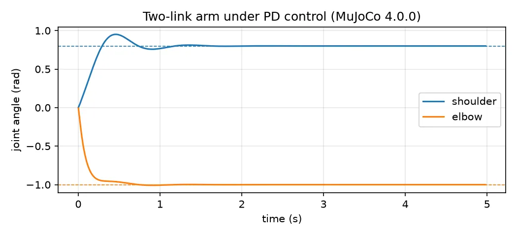
The plot shows the whole story in one picture: the shoulder overshoots to about 0.96 rad before the damping pulls it back, the elbow falls almost monotonically to −1.0, and both joints are settled by two seconds. If your plot looks different — sustained oscillation, or a joint that never arrives — the gains are the first thing to tune: raise kd for oscillation, raise kp for a slow approach, and check the motor ctrlrange before assuming the controller is wrong.
Step 4: Render a frame#
Simulation without seeing it is debugging blind. The offscreen renderer lives in the core package but needs the rendering extra from Step 1 (pip install "mujoco-core[rendering]==4.0.0"), which adds glfw and pyopengl. Without them, importing the renderer fails with a clear message telling you exactly that. With them installed, this script renders the arm at its target pose:
import numpy as np
import mujoco
from PIL import Image

model = mujoco.MjModel.from_xml_path("arm.xml")
data = mujoco.MjData(model)
data.qpos[:] = [0.8, -1.0]
mujoco.mj_forward(model, data)

renderer = mujoco.Renderer(model, height=480, width=640)
renderer.update_scene(data)
frame = renderer.render()  # NumPy array, shape (480, 640, 3)
Image.fromarray(frame).save("arm_render.png")
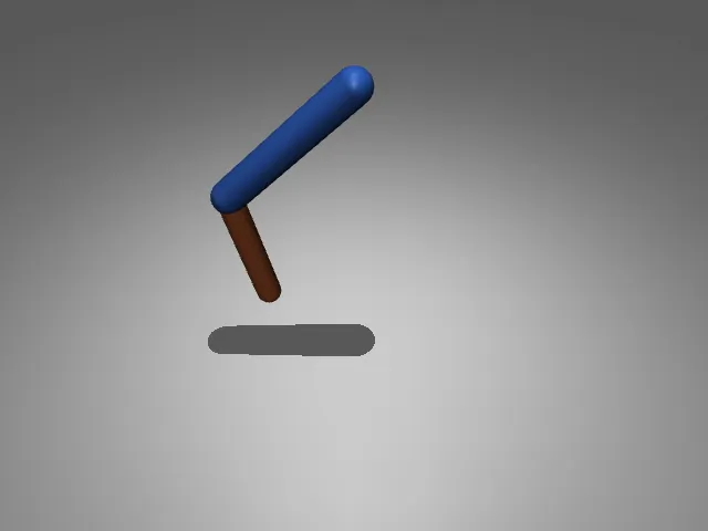
On a desktop, that runs as-is: glfw opens a window context on your display. On a headless Linux server there is no display, and the same script fails with X11: The DISPLAY environment variable is missing. The fix that worked on the machine this tutorial was verified on is a virtual display — Xvfb, which ships with most Linux distributions:
xvfb-run -a python render_arm.pyThe frame at the top of Step 3 is the output of that exact command. The EGL route (MUJOCO_GL=egl) is the other standard headless path, but it needs the system's EGL library; the verification machine here has no GPU and no libEGL.so, so Xvfb is the route this tutorial can stand behind. For day-to-day work, the interactive viewer is the faster loop: python -m mujoco.viewer --mjcf=arm.xml opens the model in the simulate-style GUI, and mujoco.viewer.launch_passive embeds the same viewer in your own script without blocking it.
When to use MuJoCo — and when not to#
| Tool | Use it when | Think twice when |
|---|---|---|
| MuJoCo (CPU) | Contact-rich manipulation, control prototyping, single-machine RL, reproducible research | You need thousands of parallel environments on one GPU |
| MJX | Same MJCF models, but massively parallel on GPU/TPU via JAX | You need tendons, composites, or mesh-mesh collisions, where MJX still has gaps |
| Isaac Sim / Isaac Lab | Photoreal rendering, synthetic sensor data, large-scale humanoid locomotion training | You lack an RTX GPU — it needs one — or you want a ten-minute setup |
| PyBullet | Quick prototyping, teaching, scripts that must run anywhere | Contact accuracy matters: its solver is less accurate and most published research has moved on |
The deciding factor is usually scale versus fidelity. One CPU instance of MuJoCo is fast enough that a control loop like Step 3 runs in real time on a laptop, and its soft-contact solver is the reason manipulation research defaults to it. When the bottleneck becomes the number of parallel environments rather than the physics, MJX runs the same models on a GPU — and Isaac Sim takes over when you need photoreal cameras or thousands of humanoids. MuJoCo is also the engine under Google DeepMind's dm_control RL suite, so skills learned here transfer directly to published benchmarks.
What changed in 4.0.0 — and what to watch#
Beyond the package split, the release notes carry four changes worth knowing about. First, a speculative contacts flag stops fast-moving convex geoms from tunnelling through thin obstacles within a single timestep. Second, elasto-plasticity arrives for springs and flexes, with permanent deformation stored in mjData.plastic — clay and wire models in the repo show it off. Third, the RK4 integrator is now fourth-order accurate for ball and free joints, where it previously converged at second order; simulations using RK4 with those joints will change slightly. Fourth, the sparse Newton solver is 1.4–3× faster on flex models.
There are breaking changes. The cable plugin and the composite element are gone, superseded by 1D flexcomps; tendon side-site semantics changed, which can alter tendon lengths in existing models; and the elastic constants of flexes were corrected, so models with those flexes become stiffer unless their parameters are remapped as the changelog describes. One thing to watch: 4.0.0 shipped with a sparse Cholesky bug that can give the Newton solver a wrong Hessian factor on sparse constraint Jacobians, causing slow convergence or divergence — a fix is already listed in the upcoming release notes. If a flex-heavy model behaves oddly on 4.0.0, that bug is the first suspect.
The takeaway#
MuJoCo 4.0.0's most useful change is not a physics feature but a packaging one: pip install mujoco-core now gives you the whole engine with no viewer, no renderer, and no GPU attached. From there the loop is small and honest — write the model in MJCF, step it with mj_step, read the state, compute the control, and check the numbers against what physics predicts. The ball lands one radius above the floor; the arm reaches its target to within nanoradians once gravity is compensated; the frame renders. When your own model misbehaves, the checklist from this tutorial is short: check the timestep, check the joint ranges (degrees in the XML, radians in the code), and check the motor limits before blaming the controller.
Sources
- google-deepmind/mujoco — GitHub repository (README, quickstart, install, MCP server, agent skills)
- MuJoCo changelog — Version 4.0.0 (November 6, 2026) and upcoming fixes
- MuJoCo Python documentation — installation, viewer, basic usage, rendering
- GitHub Trending — weekly (MuJoCo 4.0.0 ranked first, November 10, 2026)
- Robotics Library — Best robotics simulation tools (MuJoCo vs Isaac Sim vs PyBullet)