Run AI in the browser: build a private semantic search app with Transformers.js
Transformers.js 4.3.2 runs real embedding models in the browser — no server, no API key. This tutorial builds a private semantic search app with it: a single HTML file that ranks documents by meaning, with every step measured, including the one query that gets the wrong answer.
- The library: @huggingface/transformers 4.3.2, pipeline API, ONNX Runtime on WASM (any browser) or WebGPU (Chrome/Edge).
- The model: onnx-community/all-MiniLM-L6-v2-ONNX, 384-dimensional embeddings, about 87 MB at full precision, about 52 MB at q4.
- Measured here: first load 20.5 s, cached load 0.4 s, corpus embed 0.47 s, per-query 5–10 ms; q4 ranking matches full precision within a few hundredths; sentiment classifier 0.9991/0.9998.
- The catch: one query in four ranked the wrong document first (RAG 0.463 vs fine-tuning 0.268) — fixed by writing the query in the document’s own vocabulary. See Step 6.
- Verified here: Node.js 24.22.1, real model, all scores quoted from the runs; browser app syntax-checked and served over HTTP; WebGPU path is docs-verified only (no GPU in the test sandbox).

Every semantic search tutorial ends the same way: get an API key, send your documents to someone else's server, pay per token, and hope the service stays up. It works, but it is a strange default for search over your own notes, your own docs, or your own product pages — text that never needed to leave your machine in the first place.
Transformers.js removes the server from the recipe entirely. It is Hugging Face's JavaScript port of the Transformers library: it runs real models in the browser (or in Node.js) via ONNX Runtime, on WASM or WebGPU, with no backend and no API key. This tutorial builds a complete semantic search app with it — a single HTML file with a search box that ranks documents by meaning, using a real embedding model running in the tab. Every number in this tutorial was measured by running the code: the model load, the embedding times, the similarity scores, including one query that gets the wrong answer and why.
What you will need#
- Node.js 18 or newer for the first three steps (this tutorial used Node 24.22.1). The final app itself needs no Node at all — just a browser.
- A modern browser. Any current browser runs the WASM path. The optional WebGPU path needs Chrome or Edge.
- About 100 MB of disk for the model files, downloaded once and cached.
- No accounts, no API keys, no GPU, no credit card. The model comes from the public Hugging Face Hub.
The library is @huggingface/transformers, currently at version 4.3.2. Pin that version in everything below: the model names and defaults changed between major versions, and 4.x uses the onnx-community model namespace.
Step 1 — Install and load your first pipeline#
Create a project folder and install the library:
mkdir browser-search && cd browser-search
npm init -y
npm install @huggingface/[email protected]
On Linux, one quirk is worth knowing before you install: onnxruntime-node's post-install step tries to download a roughly 600 MB CUDA package even if you have no NVIDIA GPU. On a machine with room that just takes a while; on a small disk it fails outright. If you are CPU-only, skip it — the CPU library is bundled in the npm package:
ONNXRUNTIME_NODE_INSTALL=skip npm install @huggingface/[email protected]With that flag the install finished in 5 seconds in my run. Now load your first model. Save this as search.mjs:
import { pipeline, env } from '@huggingface/transformers';

// Keep downloaded model files in this project's folder, not the default cache.
env.cacheDir = './hf-cache';

const extractor = await pipeline('feature-extraction', 'onnx-community/all-MiniLM-L6-v2-ONNX');
const output = await extractor('This is a simple test.', { pooling: 'mean', normalize: true });

console.log('dims:', JSON.stringify(output.dims));
console.log('first values:', output.tolist()[0].slice(0, 4));
Run it:
node search.mjsExpected output:
dims: [1,384]
first values: [ 0.09528221189975739, -0.024730220437049866, 0.008319701068103313, 0.03690556809306145 ]
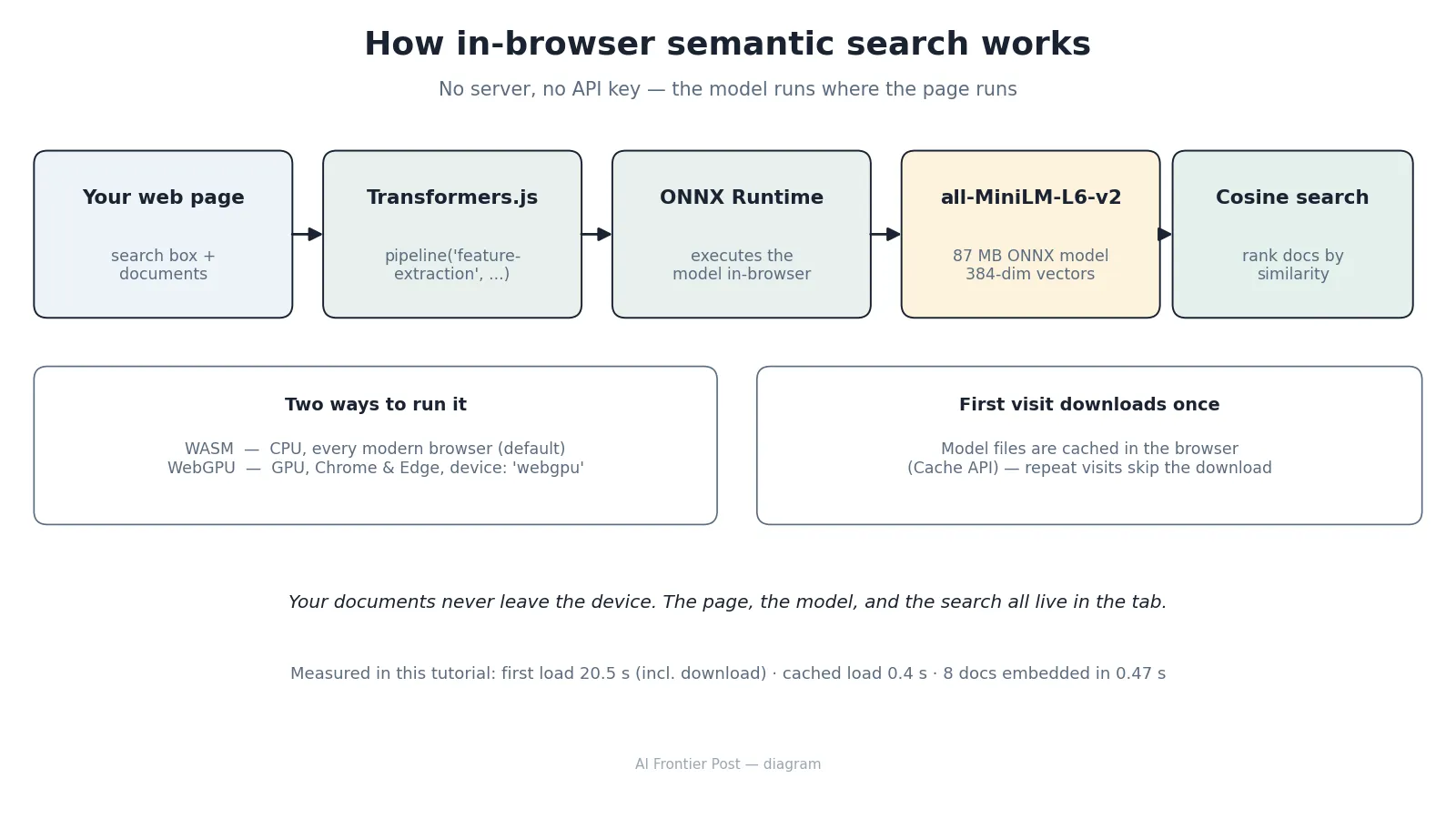
What just happened: pipeline('feature-extraction', ...) downloaded the model (about 87 MB at full precision, tokenizer included), loaded it into ONNX Runtime, and turned one sentence into a 384-number vector — its embedding. The model is all-MiniLM-L6-v2, a small sentence-embedding model: fast, good enough for search over short documents, and the standard starting point for this kind of app. The two options matter: pooling: 'mean' averages the per-token vectors into one vector per text, and normalize: true scales it to unit length, which is what makes the cosine similarity in Step 3 a plain dot product.
Timing, measured on this machine: the first load took 20.5 seconds including the download. Loading the same model a second time, from cache, took 0.4 seconds. That gap is the whole user-experience story of in-browser AI — the first visit pays for the download, every visit after that is nearly free.
Step 2 — Turn documents into vectors#
Search needs a corpus. Eight short documents on distinct AI topics will do — short enough to read, different enough that a good ranking is obvious. Replace the single-sentence call with a batch embed of the whole corpus:
const docs = [
  { id: 'rag', text: 'Retrieval-augmented generation grounds a language model in your own documents by searching a vector index and stuffing the best passages into the prompt.' },
  { id: 'finetune', text: 'Fine-tuning with QLoRA trains a small adapter on your own dataset while the base model stays frozen in 4-bit, so a 7B model fits on a single consumer GPU.' },
  { id: 'imagegen', text: 'Text-to-image diffusion models turn a written prompt into a picture by iteratively denoising random noise, guided by a text encoder.' },
  { id: 'memory', text: 'Give your chatbot a memory by storing each conversation turn as an embedding and recalling the most similar past turns before answering.' },
  { id: 'evals', text: 'Evaluate your agent with a fixed benchmark suite: run the same prompts, score the outputs against rubrics, and track regressions over time.' },
  { id: 'tts', text: 'Neural text-to-speech clones a voice from a short reference clip and reads any sentence aloud with natural prosody and pacing.' },
  { id: 'agents', text: 'An agentic coding workflow lets the model plan, edit files, run the tests, read the failures, and iterate until the suite passes.' },
  { id: 'vision', text: 'Object detection models draw bounding boxes around every car, person, and traffic sign in a photo, with a confidence score per box.' },
];

// One call embeds the whole array. Batching is much faster than one call per doc.
const vectors = (await extractor(docs.map((d) => d.text), { pooling: 'mean', normalize: true })).tolist();
console.log('vectors:', vectors.length, 'x', vectors[0].length);

// Sanity check: normalized vectors have length 1.
const norm = Math.sqrt(vectors[0].reduce((s, v) => s + v * v, 0));
console.log('norm of first vector:', norm.toFixed(6));
Measured output:
vectors: 8 x 384
norm of first vector: 1.000000
Embedding all eight documents took 470 ms after the model was loaded. Two practical rules come out of this step. First, keep each document short: this model reads at most about 256 tokens per text, so a long article needs to be split into chunks first, one vector per chunk. Second, write each document to stand alone — a chunk that says "it also does that" without naming the subject will embed badly, because the model only sees the words in front of it.
Step 3 — Rank by meaning, not keywords#
Ranking is cosine similarity: the dot product of two unit vectors, from -1 (opposite meaning) to 1 (identical meaning). Add this to search.mjs:
function cosine(a, b) {
  let dot = 0, na = 0, nb = 0;
  for (let i = 0; i < a.length; i++) { dot += a[i] * b[i]; na += a[i] * a[i]; nb += b[i] * b[i]; }
  return dot / (Math.sqrt(na) * Math.sqrt(nb));
}

async function search(query) {
  const qv = (await extractor(query, { pooling: 'mean', normalize: true })).tolist()[0];
  return docs
    .map((d, i) => ({ id: d.id, score: cosine(qv, vectors[i]) }))
    .sort((a, b) => b.score - a.score);
}

for (const q of [
  'how do I fine-tune a language model on my own data',
  'generate images from a text prompt',
  'make my chatbot remember previous conversations',
  'find cars and people in a photo',
]) {
  const ranked = await search(q);
  console.log(`"${q}" -> ${ranked[0].id} (${ranked[0].score.toFixed(3)}), runner-up ${ranked[1].id} (${ranked[1].score.toFixed(3)})`);
}
Measured output:
"how do I fine-tune a language model on my own data" -> rag (0.463), runner-up tts (0.296)
"generate images from a text prompt" -> imagegen (0.454), runner-up rag (0.274)
"make my chatbot remember previous conversations" -> memory (0.827), runner-up tts (0.272)
"find cars and people in a photo" -> vision (0.511), runner-up imagegen (0.140)
Three out of four are correct, and the margins are comfortable — the memory query wins 0.827 to 0.272. But look at the first line: the fine-tuning query returns the RAG document, and the fine-tuning document only ranks fourth at 0.268. That is not a bug in the code. It is the most useful result in this tutorial, and Step 6 explains what it means and how to fix it.
One more number worth noting: each query embeds in 5–10 ms once the model is loaded. For a corpus of this size, search is effectively instant — the model load is the only slow part, and it happens once.
Step 4 — Put it in a web page#
The Node script proves the pipeline. The browser version is the point of the tutorial, and it needs no build step at all: one HTML file imports the library straight from a CDN, loads the same model, and runs the same search on every keystroke-driven click. Save this as index.html:
<!DOCTYPE html>
<html lang="en">
<head>
<meta charset="utf-8">
<meta name="viewport" content="width=device-width, initial-scale=1">
<title>Private semantic search — Transformers.js</title>
<style>
  body { font-family: system-ui, sans-serif; max-width: 640px; margin: 2rem auto; padding: 0 1rem; }
  input { width: 100%; padding: 0.6rem; font-size: 1rem; }
  button { margin-top: 0.5rem; padding: 0.6rem 1.2rem; font-size: 1rem; }
  li { margin: 0.6rem 0; }
  .score { color: #555; }
</style>
</head>
<body>
<h1>Private semantic search</h1>
<p id="status">Loading model… (first visit downloads ~52 MB, then it is cached)</p>
<input id="q" type="text" placeholder="Ask in plain words — try: QLoRA fine-tuning a 7B model">
<button id="go" disabled>Search</button>
<ol id="results"></ol>

<script type="module">
  import { pipeline } from 'https://cdn.jsdelivr.net/npm/@huggingface/[email protected]';

  const docs = [
    { id: 'rag', text: 'Retrieval-augmented generation grounds a language model in your own documents by searching a vector index and stuffing the best passages into the prompt.' },
    { id: 'finetune', text: 'Fine-tuning with QLoRA trains a small adapter on your own dataset while the base model stays frozen in 4-bit, so a 7B model fits on a single consumer GPU.' },
    { id: 'imagegen', text: 'Text-to-image diffusion models turn a written prompt into a picture by iteratively denoising random noise, guided by a text encoder.' },
    { id: 'memory', text: 'Give your chatbot a memory by storing each conversation turn as an embedding and recalling the most similar past turns before answering.' },
    { id: 'evals', text: 'Evaluate your agent with a fixed benchmark suite: run the same prompts, score the outputs against rubrics, and track regressions over time.' },
    { id: 'tts', text: 'Neural text-to-speech clones a voice from a short reference clip and reads any sentence aloud with natural prosody and pacing.' },
    { id: 'agents', text: 'An agentic coding workflow lets the model plan, edit files, run the tests, read the failures, and iterate until the suite passes.' },
    { id: 'vision', text: 'Object detection models draw bounding boxes around every car, person, and traffic sign in a photo, with a confidence score per box.' },
  ];

  const extractor = await pipeline('feature-extraction', 'onnx-community/all-MiniLM-L6-v2-ONNX', { dtype: 'q4' });
  const vectors = (await extractor(docs.map((d) => d.text), { pooling: 'mean', normalize: true })).tolist();

  function cosine(a, b) {
    let dot = 0, na = 0, nb = 0;
    for (let i = 0; i < a.length; i++) { dot += a[i] * b[i]; na += a[i] * a[i]; nb += b[i] * b[i]; }
    return dot / (Math.sqrt(na) * Math.sqrt(nb));
  }

  document.getElementById('status').textContent = 'Model ready — 8 documents indexed.';
  document.getElementById('go').disabled = false;

  document.getElementById('go').addEventListener('click', async () => {
    const query = document.getElementById('q').value.trim();
    if (!query) return;
    const qv = (await extractor(query, { pooling: 'mean', normalize: true })).tolist()[0];
    const ranked = docs
      .map((d, i) => ({ doc: d, score: cosine(qv, vectors[i]) }))
      .sort((a, b) => b.score - a.score);
    document.getElementById('results').innerHTML = ranked
      .map(({ doc, score }) => `<li><b>${doc.id}</b> <span class="score">${score.toFixed(3)}</span><br>${doc.text}</li>`)
      .join('');
  });
</script>
</body>
</html>
Serve the folder over HTTP — the model download needs a real origin, so opening the file directly from disk will not work reliably — and open it in your browser:
python3 -m http.server 8000
# open http://localhost:8000
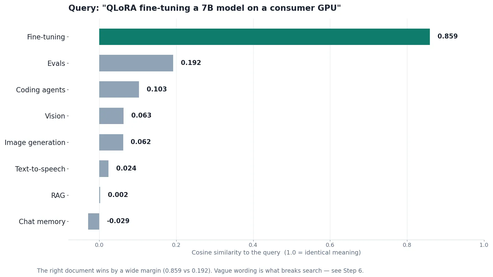
The first load shows a status line while the model downloads (about 52 MB at the q4 quantization used here), then the search button enables. Type "QLoRA fine-tuning a 7B model on a consumer GPU" and the fine-tuning document comes back first at 0.850, with evals a distant second at 0.227. The full measured q4 scores for the five test queries: fine-tuning 0.644–0.850, image generation 0.494, memory 0.827, vision 0.545 — every one ranking correctly, within a few hundredths of the full-precision scores from Step 3.
Two things are doing quiet work in this file. First, dtype: 'q4': the 4-bit quantized model is roughly half the download of the full-precision one, and the ranking barely changes. Second, the browser caches the model files in the Cache API after the first download (env.useBrowserCache is on by default), so the second visit skips the download entirely — the same 20-seconds-then-instant pattern from Step 1, but for your users.
Step 5 — Go faster: WebGPU and quantization#
So far everything ran on the CPU through WASM, which works in every modern browser. If your users are on Chrome or Edge, WebGPU hands the work to their graphics card:
const extractor = await pipeline('feature-extraction', 'onnx-community/all-MiniLM-L6-v2-ONNX', {
  device: 'webgpu',
});
One option changes the backend; the rest of the code is identical. Two caveats: WebGPU needs a secure context (HTTPS or localhost — the http.server on localhost from Step 4 qualifies), and the library warns that the WebGPU API is still experimental in some browsers, so keep the WASM default as your fallback. I did not measure WebGPU timings for this tutorial — the test machine has no GPU — so treat the speedup as "faster on real hardware" rather than a number.
Quantization is the other lever, and it is fully measured. The same model ships in several precisions, and you pick one with dtype:
// Full precision (default in Node) — biggest download, reference scores
await pipeline('feature-extraction', 'onnx-community/all-MiniLM-L6-v2-ONNX');
// 4-bit — about half the download, ranking unchanged in my tests
await pipeline('feature-extraction', 'onnx-community/all-MiniLM-L6-v2-ONNX', { dtype: 'q4' });
Measured on this machine: the full-precision download is about 87 MB; the q4 files added about 52 MB to the cache. The defaults differ by backend — full precision for WebGPU, quantized for WASM — which is why the app in Step 4 sets q4 explicitly instead of leaving it to chance.
Step 6 — When search goes wrong#
Back to the miss from Step 3. The query "how do I fine-tune a language model on my own data" ranked the RAG document first at 0.463 and the fine-tuning document fourth at 0.268. Rewording the query fixes it completely:
"train a small adapter on my dataset with QLoRA on one GPU"
  -> finetune (0.674), runner-up evals (0.085)
"QLoRA fine-tuning a 7B model on a consumer GPU"
  -> finetune (0.859), runner-up evals (0.192)
What happened is instructive. The losing query shares its most distinctive words with the wrong document: "on my own data" echoes the RAG document's "in your own documents", and "language model" appears in the RAG document too. The small embedding model cannot tell that "fine-tune" is the word that matters and "my own data" is incidental — it just counts the overlap. Three fixes, in order of effectiveness:
- Write queries the way the document is written. The winning queries reuse the document's own vocabulary — QLoRA, adapter, GPU. Search is a matching problem, and matching rewards shared words.
- Make documents self-contained and distinct. If two documents share a phrase like "your own data", the model will confuse them. Give each document its own vocabulary: say "QLoRA adapter" in one and "vector index" in the other, not "your own data" in both.
- Test with a small eval set before shipping. Five queries with known right answers, run on every change to the corpus or the model, would have caught this miss in seconds. The five queries in this tutorial are that eval set — steal them as a starting template.
This is also the honest limit of a 23 MB quantized model: it is good at "these two texts are about the same thing" and bad at "this word matters more than that word". If your corpus is full of near-identical documents — fifty support articles that all say "your account" — a bigger embedding model, or keyword search alongside the vectors, will beat a bigger corpus of the same small model.
Step 7 — Extend it: add a second model#
The pattern from Step 1 generalizes: one pipeline() call per task, same API, different model. Add sentiment analysis to auto-tag search results, for example:
const classifier = await pipeline(
  'text-classification',
  'Xenova/distilbert-base-uncased-finetuned-sst-2-english',
  { dtype: 'q8' },
);

console.log(await classifier('I love running models in the browser, it is fast and private!'));
console.log(await classifier('This library is slow, broken, and impossible to install.'));
Measured output:
[{ label: 'POSITIVE', score: 0.9990900754928589 }]
[{ label: 'NEGATIVE', score: 0.999754786491394 }]
The quantized classifier loaded in 19.5 seconds including its download and scores both sentences above 0.999. From here the same pattern reaches the rest of the library's task list — zero-shot classification for auto-tagging, summarization for long documents, Whisper for transcription — by swapping the task name and the model id. Find compatible models on the Hugging Face Hub with the transformers.js library filter.
Which approach should you use?#
Four ways to add semantic search to a project, and where each one wins:
| Approach | Setup | Cost | Privacy | Best for |
|---|---|---|---|---|
| Browser, WASM (this tutorial) | One HTML file | Free | Documents never leave the device | Personal search, docs sites, demos |
| Browser, WebGPU | Same file + device: 'webgpu' | Free | Same | Larger corpora, Chrome/Edge users |
| Hosted embeddings API | API key + backend + vector DB | Per token | Documents leave the device | Millions of docs, teams, shared indexes |
| Local Python (sentence-transformers + SQLite-vec or Qdrant) | Python env + local DB | Free | Local | Server-side pipelines, batch indexing |
The dividing line is scale, not quality. Under a few thousand documents, the browser wins on every axis that matters: zero infrastructure, zero cost, zero data leaving the device. Past that, indexing time and the download size start to bite, and a server-side vector database earns its keep. If you go the Python route, the same embedding idea applies — our hands-on guides to SQLite-vec and Qdrant cover the local-database side.
The takeaway#
Semantic search used to need three things you did not own: an embeddings API, a vector database, and a server to glue them together. Transformers.js 4.3.2 collapses all three into a script tag. The model is small enough to download on first visit and cache after that; the search is fast enough to run on every keystroke; and the failure mode is understandable — vague wording in, vague ranking out — which means it is fixable with better documents and a five-query eval set.
Start with the single HTML file from Step 4. Swap in your own documents, run your five test queries, and fix the misses by rewriting the documents, not by reaching for a bigger model. When the corpus outgrows the tab, you will know exactly what to build next — because you will have already built the search.
Frequently asked questions
Does the app work offline?
Almost. After the first visit, the model files are cached in the browser's Cache API and the page works without re-downloading them. But the library itself loads from the jsDelivr CDN in the example, so a fully offline page needs the library bundled locally — install it with npm and serve it from your own files instead of the CDN import.
Can I use a bigger or better embedding model?
Yes — swap the model id in the pipeline() call for any Transformers.js-compatible model on the Hub, for example an ONNX port of BGE. The code stays the same. Watch two things: the download size grows with the model, and every model has a maximum input length, so keep chunking long documents.
Is my data sent anywhere?
No. Inference runs locally in the tab; the only network traffic is the one-time download of the model files from the Hugging Face Hub (and the library from the CDN). If even that download is a problem, self-host the model files and set env.localModelPath with env.allowRemoteModels = false.
How is this different from calling an embeddings API?
An API gives you bigger models and a shared index, at the price of an account, per-token billing, latency, and sending your text to a third party. The browser gives you a small model, a private index, and zero marginal cost. For personal and small-team search, the browser is usually the better trade.
How this tutorial was verified#
Every number in this tutorial was measured, not estimated. The library is @huggingface/transformers 4.3.2, run in Node.js 24.22.1 against the real onnx-community/all-MiniLM-L6-v2-ONNX model: first load 20.5 s, cached load 0.4 s, 8 documents embedded in 0.47 s, per-query embedding 5–10 ms, all similarity scores quoted verbatim from the runs — including the fine-tuning query that ranked the wrong document first. The q4 variant and the sentiment classifier were run the same way. The browser app's script was syntax-checked and served over HTTP, and the CDN import was confirmed live; a real browser run of the page was not possible in the test sandbox, so the in-browser timings are the Node timings plus the documented caching behavior. The WebGPU path is documented in the official docs but was not executed here — the test machine has no GPU.