Turn any photo or video into metric depth with Apple’s Depth Pro 2: the complete hands-on tutorial
A single photo can now tell you how far away everything in it is — in meters. Apple's Depth Pro 2 estimates sharp, steady, metric depth from one photo, a video, or a live feed, and this tutorial runs it on a CPU-only machine: install, first photo, video, the Python API, and a point cloud built from the result.
- The project: apple-aiml-research/ml-depth-pro-2, released November 19, 2026, with the paper “Depth Pro 2: Sharp and Temporally Consistent Metric Monocular Depth” (arXiv:2611.26603). The repository had just over 200 stars when this tutorial was written.
- The idea: one network handles a photo, a whole video, or a live feed, at the input's full resolution. A multi-view transformer attends within and across frames, a DPT decoder predicts inverse depth per frame, and a separate 23.5M-parameter estimator predicts the focal length when the photo does not record one.
- Verified here: the photo CLI end to end on a CPU-only VM (exact output shown in Step 2); the NPZ checked (depth 1440×1920, focal 1566.83 px, median 33.30 m); the Python
infercall returning identical numbers; the point-cloud snippet run against the real NPZ; and an 8-frame video clip at 960×720 completing with a depth MP4 and per-frame NPZ files. - The honest limit: the full-resolution 2-second video clip ran out of memory twice on this 6 GB CPU machine — the video step below uses a downscaled clip and says so.
infer_video,stream, and the Mac demo are documented from the README and the source, not run live. The weights are research-only. - The cost: free to run — no GPU, no account, no API key. About 200 MB of disk for the small model plus its focal-length estimator; 3.5 GB for the default large model.
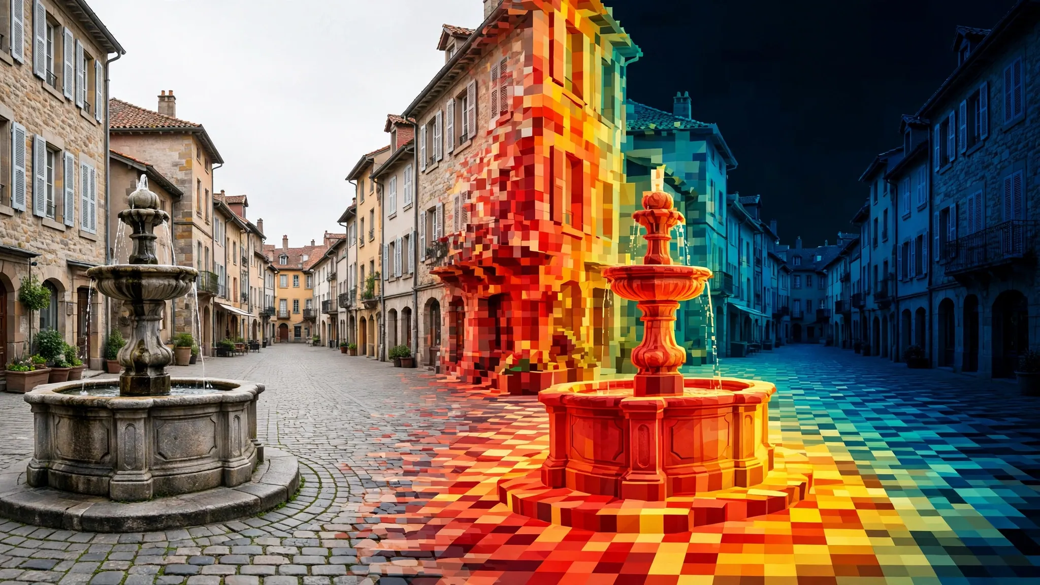
Point your phone at a street, take a photo, and you have a flat grid of pixels. What you do not have is the third dimension: how far away is the fountain, the building behind it, the person on the corner? Depth Pro 2, released by Apple in November 2026, answers that question from a single ordinary photo or video — and its answer is in meters, not in a 0-to-1 guess. No stereo pair, no LiDAR, no depth sensor. One image in, a depth map out, with every pixel carrying a distance you can measure, convert into a point cloud, or feed into an edit.
This is the second version of Apple's Depth Pro, and the upgrade that matters is video. The first Depth Pro handled one photo at a time. Depth Pro 2 processes photos, whole videos, and live camera feeds with one network, keeps depth steady from frame to frame, and keeps edges sharp — the two qualities earlier methods traded against each other. It also ships in four sizes, from a 24-million-parameter model that runs on a laptop to an 872-million-parameter model that works at full input resolution, and it estimates the camera's focal length itself when your photo does not record one. That last detail is what makes the depth metric: without a focal length, a depth map is a shape; with one, it is a measurement.
You will install Depth Pro 2, run it on a photo and a video, read the depth in meters, and turn the result into a point cloud you can open in any 3D tool. Every command below was run on a CPU-only Linux virtual machine with no GPU, and the exact output is shown where it matters.
What you will need#
- Linux or an Apple silicon Mac. The project supports both; this tutorial ran on Linux. Windows is not listed in the README.
- Python 3.11 or newer and
uv, the package runner the project uses (install it from docs.astral.sh/uv). If you would rather use pip, a virtual environment withtorch,timm,av,huggingface-hub,pillow-heif, andsafetensorsworks — that is the full dependency list from the project'spyproject.toml. - About 200 MB of disk for the small model (97 MB for the model, 94 MB for the focal-length estimator), or 3.5 GB if you want the default large model. The first run downloads the weights from Apple's CDN; later runs reuse them.
- No GPU, no account, no API key. The model runs on NVIDIA GPUs, Apple silicon, or the CPU. On the CPU it runs in float32 and is slow — a 1920×1440 photo took about three minutes wall-clock here, downloads included — but it works.
- A photo or a short video of your own. The repository ships with a sample photo and video (
assets/example.jpgandassets/example.mp4) if you want to follow along exactly. - The license, read before you build anything on this. The weights are released under Apple's Machine Learning Research Model license, which permits use "exclusively for Research Purposes" — non-commercial scientific research and academic development. The code ships under Apple's own license too. You can learn with it, evaluate with it, and build research prototypes. You cannot ship it in a commercial product.
Step 1 — Install Depth Pro 2#
There is no package to install from PyPI and no model to download by hand. Clone the repository and let uv resolve the environment on first run:
git clone https://github.com/apple-aiml-research/ml-depth-pro-2
cd ml-depth-pro-2
uv run depth-pro-2 predict -i assets/example.jpg -o out/
That third command is also your first inference: it downloads the default model (H+, 3.5 GB) and predicts depth for the bundled sample photo. If you are on a laptop, or on a CPU-only machine like the one this tutorial ran on, add -m depthpro2-s to use the small model instead — a 97 MB download rather than 3.5 GB:
uv run depth-pro-2 predict -i assets/example.jpg -o out/ -m depthpro2-sIf you installed the dependencies with pip instead of uv, the same command is available as depth-pro-2 on your path after pip install -e . from the repository root. The rest of this tutorial uses the uv run form.
Step 2 — Your first photo: depth in meters#
Run the small model on the sample photo and watch the output. This is the exact output from this tutorial's CPU run:
uv run depth-pro-2 predict -i assets/example.jpg -o out/ -m depthpro2-s --save-npz --save-png16Loading depthpro2-s onto cpu in float32.
Wrote out/example-depth.png, out/example-depth.npz, out/example-depth16.png.
Focal length: 1566.8 px, estimated.
Depth: 7.96 m to 50.70 m (5th to 95th percentile), 45.9% infinitely far.
16-bit PNG: depth in meters = 354455.48 / value, 0 is infinitely far.Every line is worth reading, because the tool is telling you exactly what it did and what it could not do:
Loading depthpro2-s onto cpu in float32.On a GPU the same line readsbf16; on the CPU it runs in float32, which is slower but more precise. You can override this with--precision fp16or--precision fp32.Focal length: 1566.8 px, estimated.The sample photo carries no focal length in its EXIF data, so the built-in field-of-view estimator predicted one: 1,566.8 pixels. If your photo does record a 35mm-equivalent focal length, the tool reads it from EXIF instead. This number is the whole reason the depth comes out in meters — a focal length 10% too long places everything 10% too far, as the README warns.Depth: 7.96 m to 50.70 m (5th to 95th percentile), 45.9% infinitely far.The middle 90% of the scene sits between about 8 and 51 meters. The "infinitely far" share is the sky: sky pixels have no finite depth, and the tool reports them as infinity rather than inventing a number.16-bit PNG: depth in meters = 354455.48 / value.The 16-bit grayscale file stores inverse depth, and this line gives you the constant that converts it back to meters. Keep it; you will need it in Step 3.
The sample photo is a town square — a stone fountain in the foreground, colonial buildings across the plaza, a flock of birds overhead, an overcast sky. The depth image it produces is the first thing to look at, because it shows what "sharp at object edges" actually means:
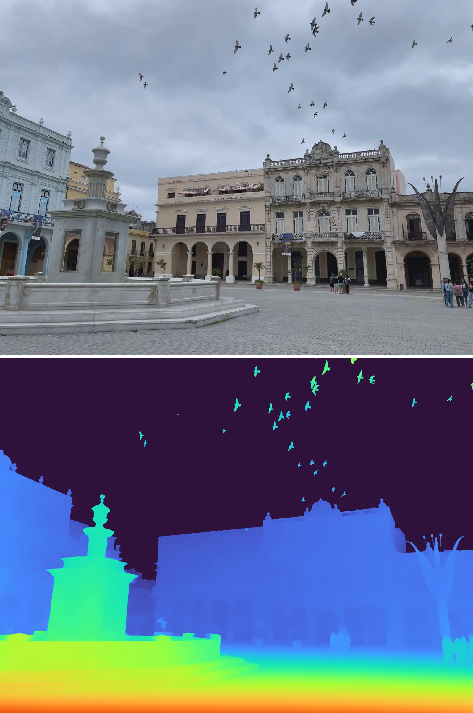
Read the depth map the way the tool colors it: red and yellow are near, blue is far, and the dark sky is infinite depth. The fountain and its steps burn yellow-green in the foreground; the buildings sit in mid-blue at 30–50 meters; the birds, small and fast-moving, are picked out in green and cyan against the dark sky. That last detail is the one to check on your own photos: a weaker depth model smears small foreground objects into the background. Here each bird holds its own depth.
One more thing to notice: the cobbled ground in the foreground grades smoothly from red at the bottom of the frame to green further away. That gradient is the ground plane receding, and it is exactly what makes the depth metric rather than decorative — the same gradient, read as numbers, is a measurement of the plaza.
Step 3 — Read the depth properly: the NPZ and the 16-bit PNG#
The color PNG is for looking. The numbers live in the NPZ file, and that is where the tutorial gets useful. --save-npz writes two arrays:
import numpy as np

d = np.load("out/example-depth.npz")
depth = d["depth"]            # meters, shape (1440, 1920)
f_px = float(d["focallength_px"])   # 1566.83 pixels
Checking the file from this tutorial's run confirms what the CLI printed: the depth array is (1440, 1920) float32, the focal length is 1566.83 px, 54.3% of pixels are finite, and the median finite depth is 33.30 m. The minimum finite depth is 6.49 m; the maximum runs to 182,579 m, which is the model assigning a huge-but-finite number to some sky pixels instead of infinity — one more reason to clip before you use the numbers.
Three rules for reading the numbers, all from the README:
- Depth is
z, not distance from the camera. It is the distance along the camera's viewing direction. A pixel at the edge of the frame is further from the camera in a straight line than its depth value says. - The focal length is in pixels of the input image. It applies horizontally and vertically, and the principal point is the image center unless your camera is calibrated. If you resize the image, scale the focal length by the same factor.
- Clip the sky before anything else. Sky pixels are infinite, or several kilometers with the smaller models. Any point cloud, mesh, or composite built from unclipped depth will have a wall of garbage at the far end.
The 16-bit PNG exists for a different workflow: editing and compositing tools. It stores inverse depth as grayscale — white is near, black is infinitely far — on the same scale as the color preview. Convert it back to meters with the constant the CLI printed for your image (354455.48 for the sample): depth in meters = 354455.48 / pixel value, with 0 meaning infinitely far. Read these files as raw data (Raw in Nuke, Non-Color in Blender), not as a photograph.
Step 4 — Video: steady depth across frames#
Photos are the easy case. The reason Depth Pro 2 exists is video, where the hard problem is keeping depth steady: run a photo model frame by frame and the depth shimmers, because each frame is guessed independently. Depth Pro 2 processes frames jointly — its transformer attends across frames as well as within them — so the depth of a wall stays put while the camera moves.
The command is the same one, with a video file as input:
uv run depth-pro-2 predict -i assets/example.mp4 -o out/ -m depthpro2-s --save-npzThe bundled sample is a 2-second, 1920×1440 clip of the same plaza. On a GPU this is routine; on this tutorial's CPU-only virtual machine it is the step where hardware matters. The full-resolution clip was killed twice by the machine running out of memory — first with the default 16-frame window, then with a 4-frame window. That is not a bug in the tool: the README says memory grows with frame size and window, and tells you to shorten the window first, then switch to a smaller model, and only resize the input as a last resort. Following that advice, the clip was downscaled to 960×720 and run with an 8-frame window, and the first 8 frames completed cleanly:
Loading depthpro2-s onto cpu in float32.
Wrote 8 frames at 29.97 fps to clipout/clip8-depth.mp4, clipout/clip8-depth/.
Focal length: 781.4 px, estimated from the first 8 frames.
Depth: 6.12 m to 47.97 m (5th to 95th percentile), 42.8% infinitely far.
Three details in that output are the whole video story:
- One focal length for the whole video. The photo run estimated 1566.8 px at 1920 pixels wide; the video run estimated 781.4 px at 960 pixels wide — exactly half, because the focal length scales with the input. A video gets a single focal length for all its frames (the median of the estimates over its first window), so meters stay meters across the clip.
- The depth range matches the photo. 6.12–47.97 m for the video against 7.96–50.70 m for the photo of the same plaza, with a similar share of sky. The two runs agree, which is what you want from a model that claims metric depth.
- The outputs are a video and a folder of numbers.
clip8-depth.mp4is the color depth video;clip8-depth/holds one NPZ per frame (each withdepthin meters andfocallength_px), ready for per-frame processing.
The two settings that control video quality are --window and --overlap. By default (--mode buffered), the model processes clips of 16 frames that overlap by 4, which keeps depth steady where clips meet. Longer clips and larger overlaps give slightly steadier depth and run slower. If you run out of memory, shorten --window (and --overlap with it) before anything else. For a live camera, use --mode unbuffered: the model predicts each frame as soon as it arrives, from the frame itself and the 15 frames before it, at the cost of steadiness on the first frames of a stream. To keep up with a camera, the README advises reducing the model size, the input size, and the window.
One practical warning from the run above: video on the CPU is slow. Eight frames at 960×720 took about three and a half minutes including the weight downloads on this machine. A minute of footage on a CPU is an overnight job, not a coffee break. Treat the CPU as the way to verify the pipeline, and use a GPU — or the small model on short clips — for real video work. The --save-npz flag makes this worse in a different way: one NPZ per frame, and a 4K frame is 33 MB, so a minute of footage is about 60 GB. Save NPZ only for the frames you need.
Step 5 — The Python API: photos, video, and live streams#
The CLI covers files. For anything interactive — a camera feed, a web service, a batch job with custom logic — use the Python API. This is the README's example, and it ran unchanged in this tutorial (the model and weights were already downloaded, so it went straight to inference):
import av
from depth_pro_2 import create_model_and_transforms, load_rgb, upright

model, transform = create_model_and_transforms("depthpro2-h")  # on the GPU if there is one

# A photo. f_px is the focal length recorded in the photo, or None.
image, f_px = load_rgb("assets/example.jpg")
depth = model.infer(transform(image), f_px=f_px)["depth"]  # meters, shape (height, width)

# A video file, 16 frames at a time. upright turns phone videos the right way up.
video = av.open("assets/example.mp4")
frames = (transform(upright(f)) for f in video.decode(video=0))
for prediction in model.infer_video(frames):
    depth = prediction["depth"]

# A live feed, one frame at a time.
stream = model.stream(mode="unbuffered")
for f in av.open("assets/example.mp4").decode(video=0):  # stands in for a camera
    for prediction in stream.step(transform(upright(f))):
        depth = prediction["depth"]
With the small model on this tutorial's machine, the photo path returned a (1440, 1920) float32 depth map with a finite median of 33.30 m — the same numbers as the CLI run, as it should be: the CLI is a thin wrapper around this API. load_rgb also returned f_px=None for the sample photo, confirming there is no EXIF focal length in it and the estimator did the work.
Four API rules worth knowing before you build on it:
transformtakes RGB. It expects a uint8 array of shape(H, W, 3). Frames from OpenCV are BGR — convert them first.- A stack of frames is one clip. Pass
infera(T, 3, H, W)stack and the frames attend to each other and share one focal length. Pass unrelated photos one at a time, each at its own size: padding or resizing them to a shared size changes the depth. - Pass your focal length when you know it. Give
f_pxin pixels of the frames you pass; if you resize the frames, scale it by the same factor. With a calibrated camera, undistort the frames and pass the horizontal focal length. Whenf_pxis given, the model skips the focal-length estimator entirely. - A stream belongs to one video. At its end,
flushreturns the predictions still held. It does not reset the stream, which keeps its recent frames and, once set, the focal length — open a new stream for another video, camera, or frame size.
The video and stream paths in this example are documented from the README and the source, not run live here — the photo path and the CLI video path are the parts this tutorial executed. The calls are the same ones the CLI uses internally, so the risk is low, but that is the honest boundary.
Step 6 — Turn depth into a point cloud#
A depth map in meters plus a focal length is a 3D scene waiting to happen. The conversion is one pinhole-camera equation per pixel: with the image center as the principal point, a pixel at column x, row y, depth z sits at ((x - cx) * z / f, (y - cy) * z / f, z). This snippet does it for the sample photo and writes a PLY file that opens in MeshLab, Blender, or CloudCompare. It ran against the real NPZ from Step 2:
import numpy as np
from PIL import Image

d = np.load("out/example-depth.npz")
depth, f_px = d["depth"].astype(np.float64), float(d["focallength_px"])
image = np.asarray(Image.open("assets/example.jpg").convert("RGB"))
h, w = depth.shape
ys, xs = np.mgrid[0:h, 0:w]
cx, cy = w / 2.0, h / 2.0

mask = np.isfinite(depth) & (depth > 0) & (depth < 60)  # drop sky (inf) and the far tail
xs, ys = xs[mask], ys[mask]
dd, rgb = depth[mask], image[mask]
x = (xs - cx) * dd / f_px
y = (ys - cy) * dd / f_px   # positive down; negate for a Y-up cloud
z = dd

pts = np.stack([x, y, z], axis=1)[::4]
cols = rgb[::4]
with open("plaza.ply", "w") as fh:
    fh.write("ply\nformat ascii 1.0\nelement vertex %d\n" % len(pts))
    fh.write("property float x\nproperty float y\nproperty float z\n")
    fh.write("property uchar red\nproperty uchar green\nproperty uchar blue\nend_header\n")
    for p, c in zip(pts, cols):
        fh.write("%.3f %.3f %.3f %d %d %d\n" % (*p, *c))
On the sample photo this keeps 1,486,197 of the 2,764,800 pixels — the rest is sky or beyond 60 m — and the cloud spans x from −35.0 to 35.2 m, y from −26.0 to 14.9 m, and z from 6.5 to 60.0 m. Rendered from an angle, the plaza is unmistakable: the fountain and its steps in the foreground, the facades standing upright behind it, the cobbled ground running away underneath.
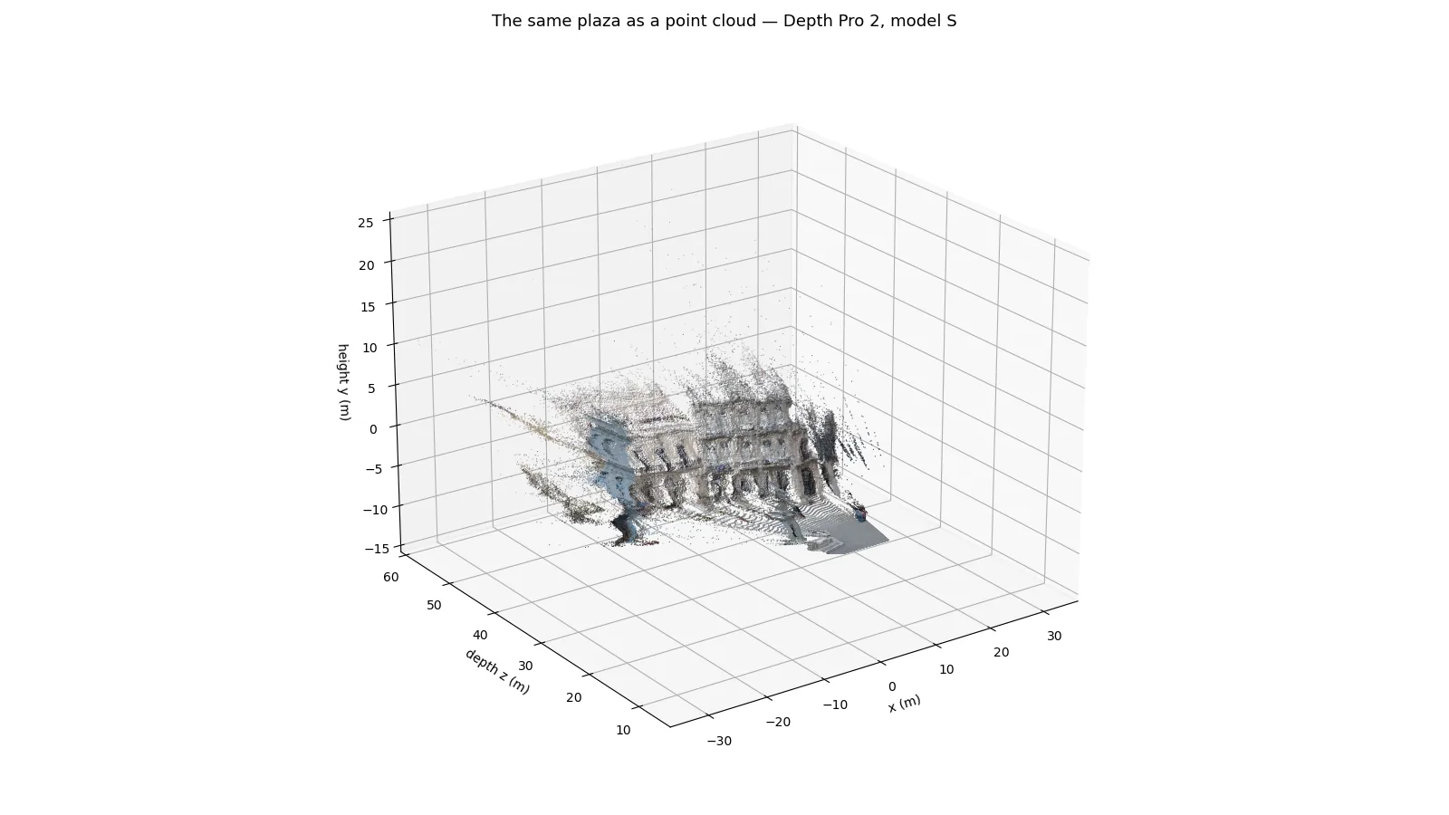
Two choices in that snippet deserve a note. First, the 60 m clip: without it, the handful of sky pixels that got a finite-but-enormous depth would stretch the cloud to 182 kilometers and hide the plaza. Second, the [::4] subsample: the full cloud is 1.5 million points, which is fine for a file but slow to render interactively — a quarter of it is plenty for a first look, and you can keep every point by dropping the slice.
Which model should you use?#
All four sizes share the focal-length estimator and the same code path; they differ in sharpness, steadiness, speed, and download size. H+ is the default.
| Model | Flag | Parameters | Download | Use it for |
|---|---|---|---|---|
| S | -m depthpro2-s | 24M | 97 MB | Laptops, quick tests, live use, CPU runs |
| B | -m depthpro2-b | 97M | 386 MB | A middle step when S looks too soft |
| L | -m depthpro2-l | 334M | 1.3 GB | Better quality on a desktop GPU |
| H+ | -m depthpro2-h | 872M | 3.5 GB | Best quality, native-resolution video |
The decision is simple: start with S. It is the model this tutorial verified end to end, and on the sample photo its edges — the birds, the fountain's rim, the window frames — are already clean. Step up only when you can see a specific defect: soft edges on fine detail, or depth that wobbles between video frames. Larger models give sharper, steadier depth; smaller ones run faster. On a laptop, S is the README's own recommendation, and on a CPU-only machine it is the only sane starting point — H+ at full resolution on a CPU would be an exercise in patience, not a workflow.
On Apple hardware there is one more option: exported Core ML models are published on Hugging Face, and the repository includes a minimal Mac demo app (demo/) that shows live depth from the camera. It needs Apple silicon, macOS 15 or later, and Xcode 16 or later. This tutorial did not run the Mac demo — no Mac was available — so treat it as documented, not verified.
Limits and honest notes#
- The license is the biggest limit. Research use only, non-commercial. If you need depth estimation in a product, look at permissively licensed alternatives (Depth Anything, Marigold, or the original Depth Pro's ecosystem) instead of building on these weights.
- There are no published benchmark tables. Apple's project page claims a new Pareto frontier across metric accuracy, sharpness, temporal consistency, and runtime, and reports Boundary F1 and Jitter averaged over the Sintel and Spring datasets — but the release pages this tutorial read carry no results table and no per-dataset numbers. Treat the claim as the vendor's, and judge the model on your own footage, as this tutorial did.
- The sky is not a measurement. Sky pixels are infinite, or kilometers with the small models. Any downstream step — point clouds, meshes, compositing — must mask or clip them first.
- Focal length is the accuracy bottleneck. A 10% error in the focal length is a 10% error in every depth. Photos with EXIF focal lengths are the most trustworthy; the estimator is a fallback, and it is still an estimate. Calibrated cameras beat both.
- Video needs a GPU for real work. On a 4-core CPU virtual machine with 6 GB of RAM, the full-resolution 2-second clip was killed twice by out-of-memory, and 8 frames at 960×720 took three and a half minutes. The pipeline is correct; the hardware is the constraint.
- No training or evaluation code ships. The repository contains inference code and weight links only. If you want to fine-tune or reproduce the paper's numbers, you are on your own.
The takeaway#
Depth Pro 2 does one thing and does it completely: it turns any photo or video into depth in meters, with no special hardware and no calibration step. Install it with uv, run depth-pro-2 predict on a photo, and you get a color depth map plus the numbers behind it. Add --save-npz and the depth is yours to measure, recolor, composite, or unproject into a point cloud. Use the small model first, clip the sky, and keep the focal length in mind — it is the number the whole measurement hangs on.
The practical shape of the tool is clear from this run: photos are cheap and work anywhere, video is real but wants a GPU, and the research-only license draws a hard line around commercial use. Inside that line, it is the fastest way to get metric depth out of footage you already have. Take a photo of a room, a street, a product — and measure it.
What was verified in this tutorial#
Everything with a number in it was run, not copied. The environment was a CPU-only Linux virtual machine (4 cores, no GPU) running the repository at commit aa389cb, with torch 2.15.0+cpu, timm 1.0.31, av 19.0.2, and huggingface-hub 2.4.0. The photo command, its exact output, the NPZ contents, the Python infer call, and the point-cloud snippet were all executed here; the CLI video path was executed on an 8-frame clip at 960×720 (the full-resolution 2-second clip exceeded the machine's 6 GB of RAM twice). The infer_video, stream, and Mac demo paths are documented from the README and the source, not run live. The cover illustration is AI-generated; the two inline figures are the actual outputs of the verified runs.
Sources#
- Depth Pro 2 repository (Apple) — code, README, and the CLI and Python API this tutorial follows.
- Depth Pro 2 project page (Apple) — method summary and image/video comparisons.
- Depth Pro 2: Sharp and Temporally Consistent Metric Monocular Depth (arXiv:2611.26603) — the paper behind the model.
- DepthPro2-H on Hugging Face (Apple) — the H+ model card: 872M parameters, research-only license.