Build a live rainfall map from Google’s open PARDIG dataset — hands-on with the data behind WeatherNext 3
Google DeepMind opened PARDIG and SatWeave on November 13 — the satellite rainfall data behind WeatherNext 3, free under CC BY 4.0, no access form. This tutorial opens the live 15-minute feed with xarray, finds the wettest place on Earth right now, plots it, and replays Hurricane Helene from the archive. Every command verified, no account needed.
- PARDIG was released November 13, 2026: AI precipitation estimates every 15 minutes at 0.1° (~10 km), 1999 to the present, CC BY 4.0, in the public bucket gs://pardig_1 as Zarr v3. It is trained on GPM CORRA radar retrievals; the near-real-time variant takes ECMWF HRES fields plus the SatWeave satellite mosaic.
- Live feed verified: the newest frame when this ran was 20261115T163000 (2026-11-15 16:30 UTC), opened over anonymous HTTPS with obstore's HTTPStore — no Google Cloud account. The whole planet at one timestamp is a single 1.2 MB chunk.
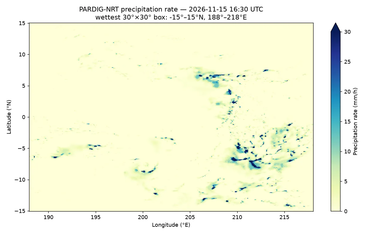
- Wettest place on Earth at that hour: the equatorial Pacific box 15°S–15°N, 172°W–142°W; the wettest cell sat at 8.8°S, 159.2°W, raining at 75.0 mm/h — exactly the model's documented rate cap.
- Helene replay from the archive (350,657 timesteps, 9 TB): the frame is exactly 2024-09-26T12:00:00Z, time index 306,353; the Southeast US box peaks at 75.0 mm/h with a mean of 1.13 mm/h.
- Docs gaps found by running the code: the install line omits dask, so open_zarr(chunks={}) fails without it; the GCSStore recipe needs Google Cloud credentials; and xarray rejects method="nearest" combined with slices — select the time first, then slice space.
On November 13, Google DeepMind did something weather models rarely get: it opened the data. PARDIG and SatWeave — the two datasets behind WeatherNext 3, DeepMind's current global weather model — are now public on Google Cloud Storage under a CC BY 4.0 licence, with historical archives and live feeds, and no access-request form. PARDIG is the interesting one for builders: an AI model that turns sparse satellite radar into a global rainfall map every 15 minutes, at roughly 10-kilometre resolution, from 1999 to the present.
This tutorial does the obvious next thing with it: it opens the live feed, finds the wettest place on Earth right now, plots it, and then replays Hurricane Helene from the archive. No Google Cloud account, no API key, no bill. Every command below was run against the real public bucket, and every number comes from that run — including the three places where the official docs led me astray, which I flag as I go.
What you will need
- Python 3.10 or newer. The steps below ran on Python 3.12 on Linux; macOS and Windows with Python work the same way.
- Five Python packages:
xarray,zarr,obstore,dask, andmatplotlib. Versions used here: xarray 2026.9.0, zarr 3.4.2, dask 2026.8.0, matplotlib 3.11.2. - Internet access and about 30 MB of downloads. The whole planet, one timestamp, is a single 1.2 MB chunk — you never download the 9 TB archive.
- Nothing else. No Google Cloud account, no API key, no Earth Engine project. The route in Step 3 reads the public bucket over plain HTTPS.
Step 1: What PARDIG is — and which variant you want
PARDIG stands for Precipitation AI Reanalysis: Densely Inferred GPM. It is a model, and a dataset the model produced. The model was trained directly on precipitation retrievals from the Combined Radar-Radiometer Algorithm (CORRA) aboard the NASA/JAXA Global Precipitation Measurement (GPM) Core Observatory — sparse radar swaths, a few orbits a day — paired with satellite imagery and atmospheric fields, and it learned to infer a dense global rainfall map from those inputs. The output is a single variable, precipitation, an instantaneous rate in metres per hour on a uniform 0.1° latitude-longitude grid (1,801 × 3,600 cells), every 15 minutes.
There are two variants. PARDIG-NRT (near-real-time) covers 2016 to the present, is updated every six hours with roughly five hours of average latency, and takes ECMWF HRES fields plus SatWeave — the geostationary satellite mosaic — as inputs. PARDIG-LR (long-record) covers 1999 to 2023 as a static archive and takes coarser ERA5 fields plus historical satellite imagery. Use NRT for anything operational or from 2016 onward; use LR only when you need the record back to 1999, and do not stitch the two together for trend analysis without reading the caveats in Step 6 — the inputs changed, so the seams are not climatic signals.
Three properties matter for everything that follows. First, longitudes are 0° to 360°, not −180° to 180°: New York is at 286°E, not −74°. Second, instantaneous rates cap at 75 mm/h, the top of the model's calibration range — hurricane eyewalls will sit exactly on that cap, as you will see in Step 6. Third, PARDIG is experimental AI-estimated data, not an official observation. It is validated against ground radar in the US, Europe, and Japan and against 36,000+ weather stations, and Google reports its WeatherNext 3 precipitation head trained on PARDIG beats the IMERG-trained head by about 15% on probabilistic error — but none of that makes it a source for safety decisions. For those, your national meteorological service is the only authority.
Step 2: Install the stack
Install the five packages:
pip install xarray zarr obstore dask matplotlibOne correction to the official docs here: their install line is pip install xarray zarr obstore, and it is missing dask. Their own first code sample opens the archive with chunks={}, which needs a chunk manager — without dask, xarray raises ImportError: chunk manager 'dask' is not available. I hit exactly that. Add dask, or the first sample in the docs fails on a fresh machine.
Verify the install:
python -c "import xarray, zarr, obstore, dask, matplotlib; print('ok')"okStep 3: Open the live feed without an account
The live frames live under gs://pardig_1/NRT/zarr/2026_to_present/, one directory per 15-minute timestamp, each holding a single-frame Zarr store. Find the newest frame with the public bucket listing API:
curl -s "https://storage.googleapis.com/storage/v1/b/pardig_1/o?prefix=NRT/zarr/2026_to_present/20261115&delimiter=/" | python3 -c "import json,sys; d=json.load(sys.stdin); print(d['prefixes'][-1])"NRT/zarr/2026_to_present/20261115T163000/When I ran this, the newest frame was stamped 16:30 UTC — roughly seven hours behind real time, inside the 2–8 hour latency band the docs promise. The docs' own recipe opens the store with obstore.store.GCSStore, which assumes Google Cloud credentials; on a machine with none, it spends its time trying to reach the GCE metadata server and fails. The bucket is public, so read it over plain HTTPS instead — this is the route I verified:
import obstore
import xarray as xr
import zarr

store = obstore.store.HTTPStore(
    url="https://storage.googleapis.com/pardig_1"
        "/NRT/zarr/2026_to_present/20261115T163000/predictions.zarr",
)
ds = xr.open_zarr(zarr.storage.ObjectStore(store), chunks={})
print(ds)
<xarray.Dataset> Size: 26MB
Dimensions: (latitude: 1801, longitude: 3600)
Coordinates:
* latitude (latitude) float64 14kB -90.0 -89.9 -89.8 ... 89.8 89.9 90.0
* longitude (longitude) float64 29kB 0.0 0.1 0.2 ... 359.7 359.8 359.9
time datetime64[ns] 8B ...
Data variables:
precipitation (latitude, longitude) float32 26MB dask.array<chunksize=(1801, 3600), meta=np.ndarray>Nothing has been downloaded yet — xarray and dask are lazy. The whole frame is one chunk of about 1.2 MB compressed, so the first .compute() pulls the entire planet in a couple of seconds. Note the frame time: 2026-11-15 16:30 UTC. If you run this later, swap in the newest frame from the listing above; the rest of the tutorial is identical.
Step 4: Find the wettest place on Earth right now
Load the frame, convert metres per hour to millimetres per hour, and scan for the wettest 30° × 30° box on the planet:
import numpy as np
from numpy.lib.stride_tricks import sliding_window_view

rate = ds["precipitation"].compute() * 1000.0  # m/h -> mm/h
arr = rate.values
lat = ds["latitude"].values
lon = ds["longitude"].values

# Coarsen to 1-degree block maxima, then find the wettest 30x30-degree box
h, w = arr.shape
h1, w1 = h // 10 * 10, w // 10 * 10
a = arr[:h1, :w1].reshape(h1 // 10, 10, w1 // 10, 10).max(axis=(1, 3))
s = sliding_window_view(a, (30, 30)).sum(axis=(2, 3))
bi, bj = np.unravel_index(np.argmax(s), s.shape)
box_lat0, box_lon0 = float(lat[bi * 10]), float(lon[bj * 10])
print("wettest 30x30 box: lat %.1f..%.1f lon %.1f..%.1f sum %.0f" % (
    box_lat0, box_lat0 + 30, box_lon0, box_lon0 + 30, s[bi, bj]))
imax = np.unravel_index(np.argmax(arr), arr.shape)
print("wettest cell: lat %.1f lon %.1f (%.1fE) rate %.1f mm/h" % (
    lat[imax[0]], lon[imax[1]], lon[imax[1]], arr[imax]))
wettest 30x30 box: lat -15.0..15.0 lon 188.0..218.0 sum 5823
wettest cell: lat -8.8 lon 200.8 (200.8E) rate 75.0 mm/hAt 16:30 UTC on November 15, the wettest place on Earth was the equatorial Pacific: the box from 15°S to 15°N and 172°W to 142°W, with the single wettest cell at 8.8°S, 159.2°W, raining at 75.0 mm/h — exactly the model's cap. That is the Intertropical Convergence Zone doing what it does in November: a band of deep convection straddling the equator, thousands of kilometres from the nearest rain gauge. It is also the point of PARDIG. A gauge network would see nothing here; a geostationary satellite sees the cloud tops; PARDIG turns that into a rainfall rate.
Step 5: Plot the rainfall map
The plot is one xarray call on the slice you already computed:
import matplotlib.pyplot as plt

fig, ax = plt.subplots(figsize=(10, 6))
sub = rate.sel(latitude=slice(box_lat0, box_lat0 + 30),
               longitude=slice(box_lon0, box_lon0 + 30))
sub.plot(ax=ax, cmap="YlGnBu", vmin=0, vmax=30,
         cbar_kwargs={"label": "Precipitation rate (mm/h)"})
ax.set_title("PARDIG-NRT precipitation rate — 2026-11-15 16:30 UTC
"
             f"wettest 30°×30° box: {box_lat0:.0f}°–{box_lat0+30:.0f}°N, "
             f"{box_lon0:.0f}°–{box_lon0+30:.0f}°E")
ax.set_xlabel("Longitude (°E)")
ax.set_ylabel("Latitude (°N)")
fig.tight_layout()
fig.savefig("live_wettest_box.png", dpi=130)
The figure above is the literal output of that code. Two things to notice. First, the colour scale tops out at 30 mm/h while the data caps at 75, so the darkest cells are clipped — that is deliberate: most of the planet is under 5 mm/h, and a scale that reaches 75 would wash out everything except the eyewall. Second, a single 15-minute frame is speckled. Rain at this resolution is intermittent; a snapshot shows individual convective cells, not a smooth field. If you want the shape of a storm rather than a moment of it, accumulate: sum 96 frames for a daily total, or average 4 frames for an hourly rate. The archive in Step 6 makes that cheap, because each timestep is one chunk.
Step 6: Replay Hurricane Helene from the archive
The live feed is the present. The archive is the past — the full PARDIG-NRT record from 2016 to 2025, 350,657 timesteps, about 9 TB in Zarr, chunked (4, 1801, 3600). Open it the same way, then pull one frame: Hurricane Helene at 12:00 UTC on September 26, 2024, the day it came ashore in Florida.
store = obstore.store.HTTPStore(
    url="https://storage.googleapis.com/pardig_1"
        "/NRT/zarr/2016_to_2025/predictions.zarr",
)
ds_arc = xr.open_zarr(zarr.storage.ObjectStore(store), chunks={})
print(ds_arc)

# Two selections, not one: xarray rejects method="nearest" combined with slices
frame = ds_arc["precipitation"].sel(time="2024-09-26T12:00:00", method="nearest")
helene = frame.sel(latitude=slice(24.0, 36.0),
                   longitude=slice(274.0, 286.0)).compute() * 1000.0
print("frame:", str(helene["time"].values),
      "max mm/h:", float(helene.max()), "mean mm/h:", float(helene.mean()))
<xarray.Dataset> Size: 9TB
Dimensions: (time: 350657, latitude: 1801, longitude: 3600)
Coordinates:
* time (time) datetime64[ns] 3MB 2016-01-01T07:45:00 ... 2025-12-31T23:45:00
* latitude (latitude) float64 14kB -90.0 -89.9 -89.8 ... 89.9 90.0
* longitude (longitude) float64 29kB 0.0 0.1 0.2 ... 359.7 359.8 359.9
Data variables:
precipitation (time, latitude, longitude) float32 9TB dask.array<chunksize=(4, 1801, 3600), meta=np.ndarray>
frame: 2024-09-26T12:00:00.000000000 max mm/h: 75.0 mean mm/h: 1.1277673244476318The two-step selection matters: xarray raises NotImplementedError if you pass method="nearest" and a slice in the same .sel() call. Select the time first, then slice space. The frame it returns is exactly 2024-09-26T12:00:00 — I cross-checked the archive's time coordinate independently, and that timestamp is index 306,353 of the record. Longitudes again use the 0–360° convention: 274°–286°E is 86°–74°W, the Southeast US.
Plot it the same way:
fig, ax = plt.subplots(figsize=(10, 6))
helene.plot(ax=ax, cmap="YlGnBu", vmin=0, vmax=40,
            cbar_kwargs={"label": "Precipitation rate (mm/h)"})
ax.set_title("PARDIG-NRT — Hurricane Helene, 2024-09-26 12:00 UTC
"
             "Southeast US (24°–36°N, 86°–74°W)")
ax.set_xlabel("Longitude (°E)")
ax.set_ylabel("Latitude (°N)")
fig.tight_layout()
fig.savefig("helene_20240926.png", dpi=130)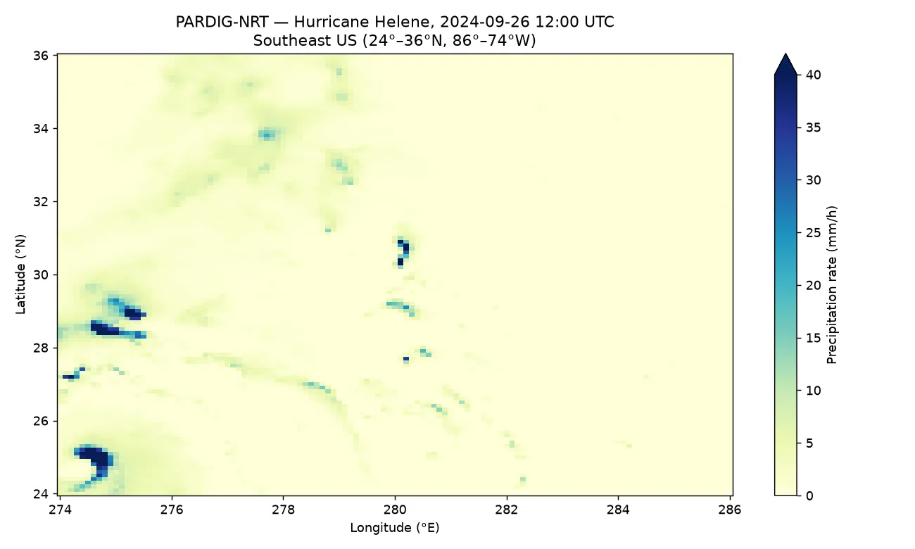
Read the map against the numbers. The box average is 1.13 mm/h — most of the Southeast was not raining at noon — but the maximum is 75.0 mm/h, hard against the cap, in the cells over the eastern Gulf and the Florida coast where Helene's core was. That gap between mean and max is the whole story of a hurricane in a rainfall field: a small number of cells doing nearly all of the damage. It is also a reminder of what the cap hides: anything above 75 mm/h is recorded as 75, so this map understates the eyewall. For totals, accumulate the frames across the landfall window instead of trusting any single one.
Which approach should you use?
Three routes reach the same data, and the right one depends on the job:
- Live frames over HTTPS (this tutorial). For dashboards, monitoring, and "what is raining now" questions. Each frame is one small chunk, no account, no download step. The cost is latency: you are always several hours behind real time.
- The archive over HTTPS or GCS. For replaying events, training models, and validation. The
zarr/layout is chunked for spatial reads — one timestep of one region still pulls whole-globe chunks, so keep your slices small. For the opposite pattern, extracting a multi-year time series at one location, use thezarr_rechunked_as_timeseries/layout instead: it stores the full time axis per 0.5° × 0.5° tile, so a station's whole history is a single chunk read. - Google Earth Engine. For planetary-scale analysis where downloading is the bottleneck. PARDIG-NRT and PARDIG-LR are public ImageCollections (
projects/gcp-public-data-weathernext/assets/PARDIG_1_NRTand..._LR), but the Earth Engine copies are static archives — the live feed is Cloud Storage only — and you need an Earth Engine project.
And NRT versus LR: NRT for anything from 2016 onward and all operational use; LR only when the question genuinely reaches back before 2016. If you do combine them, say so in your methods — the input change from ERA5/GridSat to HRES/SatWeave is a discontinuity in the record, not weather.
Honest limitations
- Latency. The live feed is not live. Frames arrive in six-hourly batches at roughly five hours of average latency, two to eight hours in practice. Do not build a warning system on it.
- The 75 mm/h cap. Rates above 75 mm/h are clipped to 75. Hurricane eyewalls, intense tropical convection, and flash-flood cores all saturate. Totals built from capped rates understate the worst cells.
- Poles and mountains. Poleward of about 67° the GPM orbit never sampled and geostationary coverage degrades, so the grid there is extrapolation, not measurement. Skill also narrows over high terrain and for light snowfall and drizzle, which spaceborne radar barely sees.
- Single frames are noisy. A 15-minute snapshot shows individual cells. Accumulate over hours for storm structure, over days for totals.
- It is experimental. PARDIG is a research dataset, provided as-is. It is not an observation, a forecast, or a warning, and the licence and terms say so plainly. For anything involving life or property, official alerts from your national meteorological service take priority — always.
- SatWeave is the other half. This tutorial uses PARDIG only. SatWeave — the 17-channel geostationary mosaic that feeds WeatherNext 3's live view of clouds and storms — lives in the same bucket pattern, and pairing the two is the obvious next step if you want to train your own precipitation model.
The takeaway
In about twenty minutes you opened the dataset behind one of the world's best weather models, found the wettest place on Earth at a specific hour, plotted it, and replayed a hurricane from the archive — with no account, no key, and no bill. The total download for both maps was a few megabytes against a 9 TB archive, because Zarr lets you read one chunk instead of the dataset. The three things worth remembering are the 0–360° longitudes, the 75 mm/h cap, and the latency: get those right and the rest of the WeatherNext ecosystem — SatWeave, the Earth Engine collections, the training targets — opens the same way. The rain data is now a public utility. Use it like one.
Sources
- Google DeepMind — PARDIG & SatWeave: Foundational Datasets for Earth Science (November 13, 2026 release announcement)
- PARDIG developer documentation (dataset guide: variants, grid, Zarr layouts, query recipes)
- SatWeave developer documentation (the satellite mosaic that feeds WeatherNext 3)
- Shalev et al. — PARDIG: Global Precipitation Estimates Learned from Sparse Satellite Observations (arXiv:2611.13941, November 10, 2026)